Electrical engineering article

Chapter 1 – Introduction: why NOMA matters for IoT

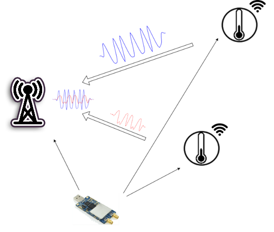
This article describes how non-orthogonal multiple access (NOMA) was implemented with software-defined radio (SDR) and tested in the lab. The starting question is whether two users can transmit at the same time in the same frequency band such that a receiver can separate both data streams—without isolating them with time slots or separate carriers.

The experiment used two independent transmitters (one SDR each) and a shared receiver. Baseband processing (filtering, synchronization, demodulation, and successive interference cancellation, SIC) was implemented mainly in GNU Radio with supporting Python; evaluation included bit error rate (BER) and dependence on the power ratio between users. The figures and curves on this page come from the same measurements.

Wireless data transmission is central to modern technical systems. In the Internet of Things (IoT) in particular, the number of connected devices is growing fast. Sensors, controllers, and embedded systems send data continuously—often at the same time and over limited radio resources.

That leads to a basic issue:

Core point: the more devices transmit, the more often collisions occur.

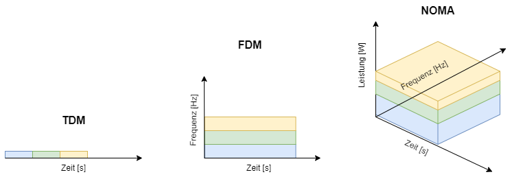
Energy-optimized IoT systems often avoid heavy protocols or acknowledgements. That saves energy but also means colliding packets are frequently lost. Classical approaches such as time-division multiplexing (TDM) or frequency-division multiplexing (FDM) try to avoid this by strictly separating users in time or frequency. Those methods scale only to a point and do not use available resources optimally.

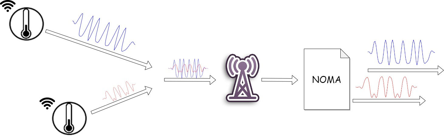
An alternative is non-orthogonal multiple access (NOMA).

Key difference: several users transmit at the same time on the same frequency.

Signals are no longer separated by disjoint channels but by receiver-side signal processing. Superposed signals are reconstructed and pulled apart deliberately.

In theory this sounds simple. In practice there are many challenges:

• Noise and interference
• Frequency and phase errors
• Different signal powers
• Synchronization issues

For NOMA to work reliably, the receiver must run complex processing steps. A central technique is successive interference cancellation (SIC), where contributions are detected step by step, reconstructed, and subtracted from the composite signal.

This article shows how such a system can be built in practice—from radio fundamentals to real signal processing with software-defined radio.

Chapter 2 – Basics: software-defined radio and data transmission

Software-defined radio (SDR)

A software-defined radio (SDR) is a radio system where as many classical hardware functions as possible are replaced by software.

In a conventional receiver many stages are fixed in hardware:

• Mixer
• Filters
• Demodulator

With an SDR the signal is digitized as early as possible and processed entirely in software afterward.

How an SDR works (simplified)

The signal path looks like this:

1. The antenna receives the RF signal.
2. The mixer shifts it to a lower frequency (IF or baseband).
3. The ADC digitizes the signal.
4. Digital signal processing handles:
   • Filtering
   • Demodulation
   • Synchronization
   • Decoding

Why this fits our setup

Crucially, the whole receiver behavior is programmable.

That is exactly why SDR pairs well with NOMA:

• Multiple superposed signals can be analyzed flexibly
• Algorithms such as SIC can be implemented directly
• Changes need no hardware redesign

Basics of digital transmission

For a radio link to work, digital data must be turned into an analog waveform.

Modulation – QPSK example

This system uses quadrature phase-shift keying (QPSK).

Properties:

• 2 bits per symbol
• Twice the data rate of BPSK
• Robust, widely used modulation

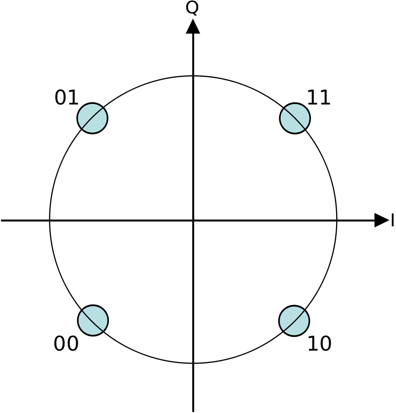
Symbols are shown as points in the complex plane:

• Real part → in-phase (I)
• Imaginary part → quadrature (Q)

Typical symbol values (I, Q):

• (1, 1)
• (−1, 1)
• (−1, −1)
• (1, −1)

Note: this yields the usual QPSK constellation diagram.

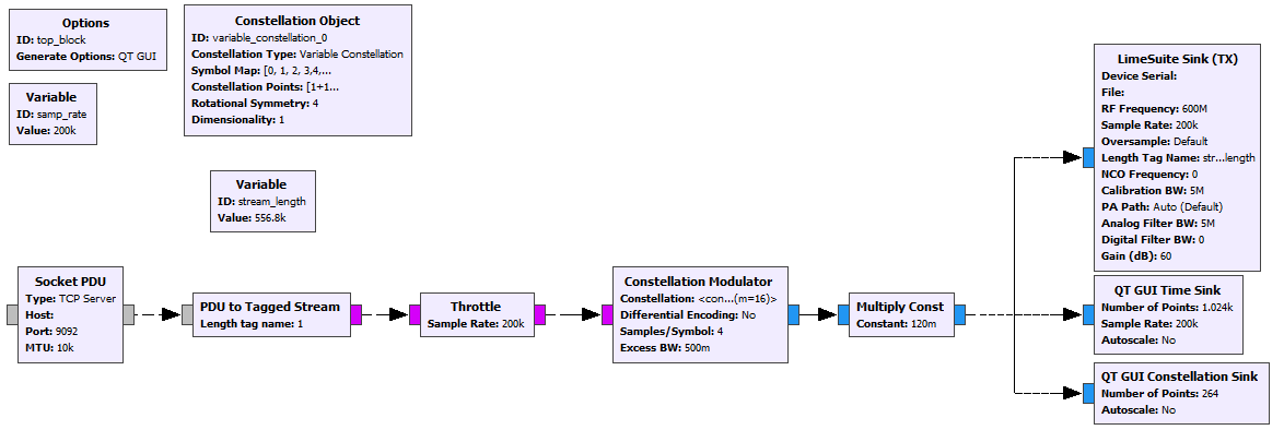
For extended QPSK (including byte packing for GNU Radio) the transmitter uses adjust_data (excerpt from BAT_NOMA_Transmitter.py):

def adjust_data(data):  # extended QPSK
    new_data = np.zeros(len(data) * 2, dtype=int)
    data_temp = np.zeros(len(data) * 2, dtype=int)
    for i in np.arange(len(data_temp)):
        data_temp[i] = data[int(i / 2)]
    for j in np.arange(len(new_data)):
        if (j % 2) == 0:
            new_data[j] = (np.uint8(np.uint8(data_temp[j] / (64)) * 16)) | (
                np.uint8(np.uint8(data_temp[j] * 4) / 64))
        if (j % 2) == 1:
            new_data[j] = np.uint8(np.uint8(np.uint8(data_temp[j] / 4) * 64) / 4) | (
                np.uint8(np.uint8(data_temp[j] * 64) / 64))
    return new_data

In the GNU Radio Constellation Object block the 16 symbol positions include four QPSK points plus several null symbols (0+0j) (see thesis appendix).

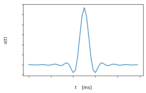
Pulse shape – root raised cosine

To transmit symbols cleanly a dedicated pulse shape is used: a root-raised-cosine (RRC) filter.

Why?

• Reduces inter-symbol interference (ISI)
• Enables clean symbol decisions
• Optimizes bandwidth use

Important: transmitter and receiver together form a matched filter (typically one RRC each); ideally ISI cancels at the sampling instants.

Receiver pulse shaping uses explicitly computed RRC coefficients and convolution to rcos (excerpt from BAT_NOMA_Receiver.py):

rrcos = np.array(
    [1, 1, 1, 0.95256299, 0.7945013, 0.56381161, 0.3173851, 0.11599391, 0.00930381])
rrcos = np.sqrt(np.concatenate((np.array([1]), rrcos, np.zeros(50 - 19), np.flip(rrcos))))
rrcos = np.fft.fftshift(np.real(np.fft.ifft(rrcos)))
rrcos = rrcos / np.sqrt(np.sum(np.square(rrcos)))
rcos = np.convolve(rrcos, rrcos)

The transmitter also uses the RRC block in GNU Radio; coefficients must match the same symbol rate / samples per symbol.

Choosing a frequency in practice

Carrier frequency strongly affects signal quality.

Typical observations:

• 2.4 GHz → heavy interference (Wi‑Fi, Bluetooth)
• Lower bands → often more stable links

Lower frequencies can mean less interference and often smaller frequency offset between devices.

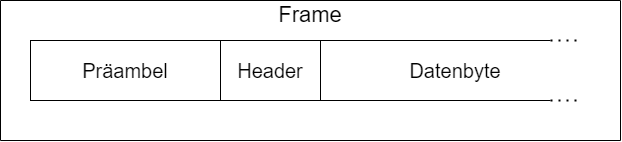
Packet structure

Transmission uses short burst packets—typical for IoT.

A packet contains:

• Preamble – synchronization and signal detection
• Header – metadata (e.g. destination)
• Payload – the actual data

Why the preamble matters

The receiver does not know when a transmission starts. The preamble is used to

• find the signal in the sample stream,
• lock the time base,
• prepare demodulation.

End-to-end data flow

Transmitter path:

1. Data → QPSK modulation
2. Pulse shaping (RRC)
3. Upconversion to carrier
4. Radiate from the antenna

Receiver path:

1. Antenna reception
2. Downconversion to baseband
3. Digitization
4. Filtering and synchronization
5. Demodulation
6. Data extraction

Why this matters for NOMA

All of the above is critical because NOMA only works if the waveform is processed very cleanly.

Even small errors cause:

• Wrong symbol decisions
• Poor interference cancellation
• User signals that cannot be reconstructed

Chapter 3 – How NOMA works

This setup treats NOMA as power-domain NOMA: users differ mainly in received power (via transmit amplitudes and path loss). The receiver exploits that ordering to decode the strongest “layer” first and peel it off step by step. The following sections formalize this picture and introduce SINR—the measurements in Chapter 7 use the same quantities.

Core idea of NOMA

Classical multiple-access schemes separate users strictly:

• TDM → different time slots
• FDM → different frequencies

NOMA does the opposite: several users transmit at the same time on the same frequency.

Separation happens only in the receiver—through signal processing.

Mathematical model

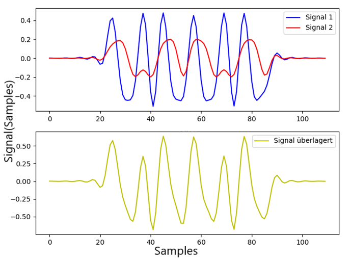
The received signal is a superposition of transmitters:

\[ x(t) = \sum_{k=1}^{N} P_k \cdot s_k(t) \]

• \(s_k(t)\): signal from user \(k\) (e.g. modulated symbols including pulse shaping)
• \(P_k\): corresponding transmit power (or amplitude factor, depending on modeling)
• \(x(t)\): composite signal at the receiver (before noise; the channel can be modeled separately)

Key point: all user signals occupy the same band and are active at the same time.

Separation by power (power domain)

The central idea in common power-domain NOMA:

Different received powers—typically from different transmit levels and/or channel attenuation.

Typical (idealized) setup:

• Farther or weaker path → higher transmit power so enough energy reaches the receiver
• Closer transmitter → lower transmit power but still detectable at the receiver

Roughly, the receiver then sees one dominant layer and one or more weaker layers underneath.

What happens at the receiver?

The received signal no longer looks like clean single-user QPSK; it is

• superposed,
• noisy,
• and distorted by channel effects.

Intuition: the weaker user acts like extra noise relative to the stronger one at first.

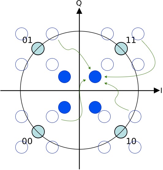
Successive interference cancellation (SIC)

The main method to separate users is successive interference cancellation (SIC).

Step-by-step flow

1. Detect the strong layer—it dominates and can initially be demodulated like a single-user link.
2. Reconstruct it—rebuild that user’s contribution from decoded symbols (including channel estimates).
3. Subtract from the received waveform.
4. The weaker layer emerges—it was hidden in the “noise” of the superposition and can now be processed.
5. Repeat for further users in order of decreasing received strength.

Why this can work

It only works if

• received powers are clearly separated,
• the dominant layer is detected reliably,
• and reconstruction is accurate.

Otherwise too much residual error remains and later demodulation stages fail.

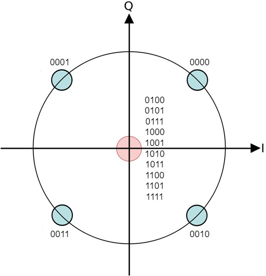
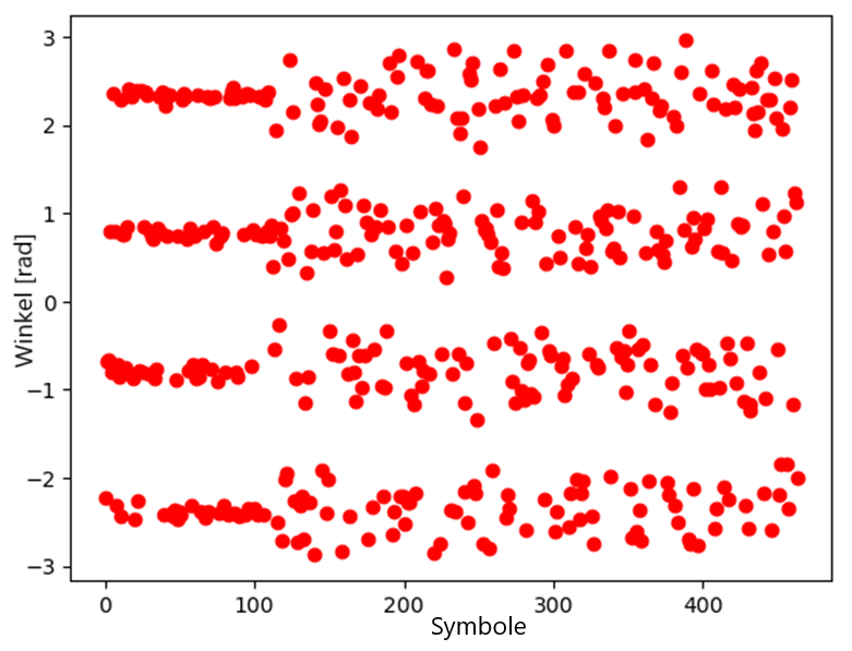
Constellation view

For QPSK the behavior is characteristic:

• without NOMA → four clear points in the I/Q plane
• with NOMA → effective symbol locations shift due to superposition

With two QPSK users, each symbol of one can combine with each symbol of the other—roughly up to 16 overlay states can appear (when both matter).

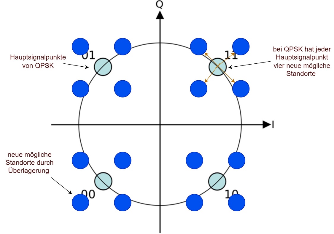
If the weaker user is too strong, points sit near decision boundaries—BER rises. If it is too weak, it disappears into the noise.

Takeaway: there is an optimal power ratio and careful power and coding design matter.

Noise and channel effects

In practice you also have:

• Thermal noise
• Path loss and fading
• Phase and frequency errors (carrier offset)

The signal is not only superposed but impaired—estimation and subtraction in SIC become harder.

SNR / SINR view

For user \(k\) an effective ratio can be written as

\[ \mathrm{SINR}_k = \frac{P_k \cdot g_k}{\sum_{i \neq k} P_i \cdot g_i + N} \]

numerator: desired signal for \(k\); denominator: interference from other users plus noise power \(N\). The \(g_k\) are (simplified) channel gains.

Strictly speaking this is a SINR; in multi-user contexts it is often loosely called SNR. Other users act like extra noise in the denominator.

Limits of NOMA

NOMA is not a silver bullet. Critical issues include:

• Unfavorable power ratio
• Poor synchronization
• Inaccurate subtraction in SIC
• Strong noise or fast time-varying channels

Then the scheme collapses quickly—errors propagate across stages.

Key takeaway

NOMA is not “just RF”—it is largely a signal-processing problem.

Success depends heavily on:

• how well the aggregate signal is estimated and synchronized,
• how precisely strong users are reconstructed and subtracted.

Chapter 4 – Signal processing: transmitter to receiver

This chapter covers the full signal path—not only what happens but how samples must be processed for NOMA to work at all.

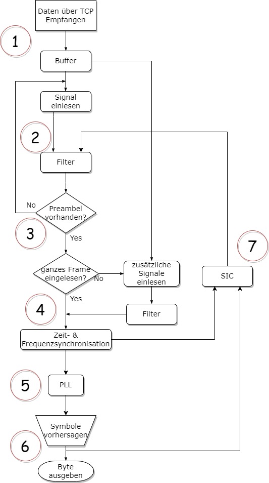
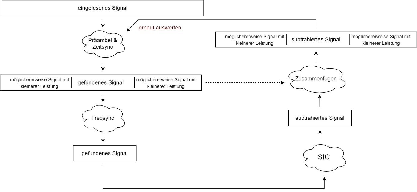
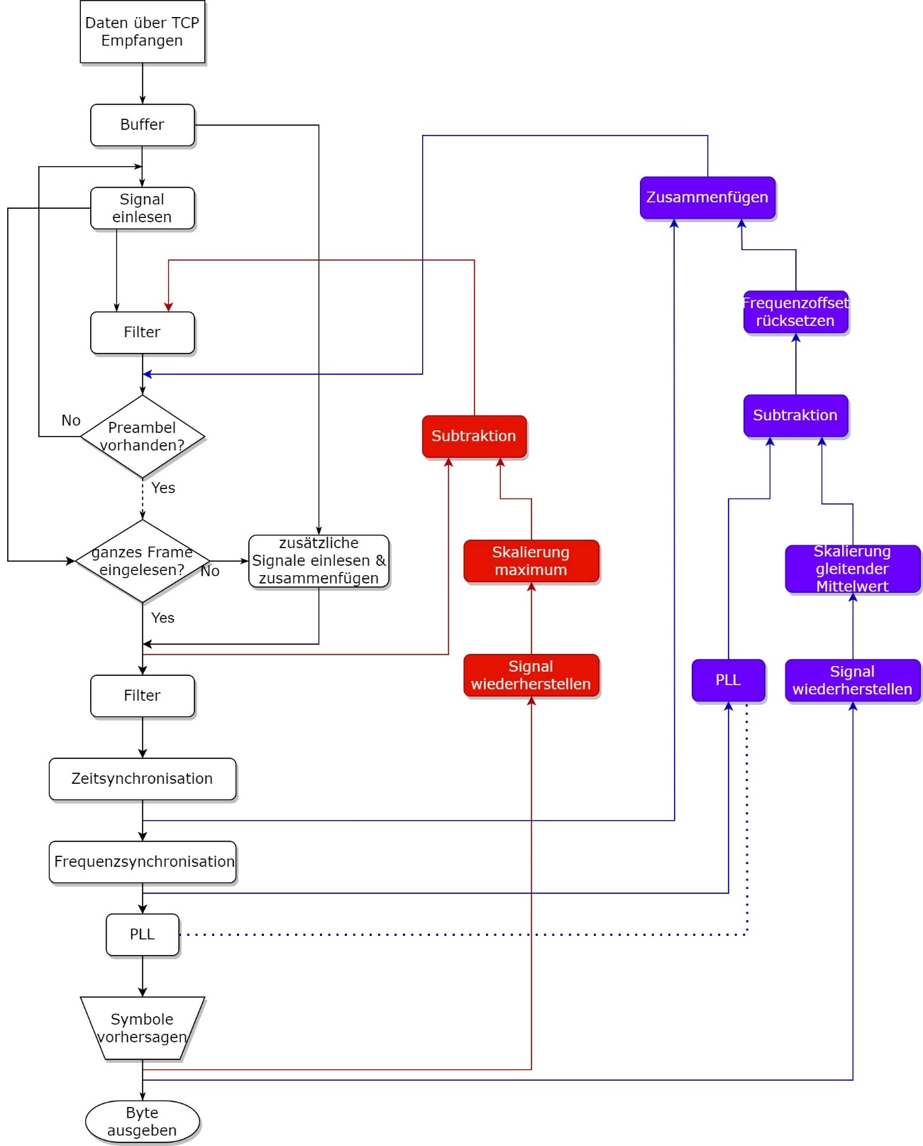
After the SDR the receiver has a continuous stream of complex baseband I/Q samples. Further steps are software-side: buffering, matched filtering (RRC), preamble search by correlation, frequency and timing alignment, downsampling to symbol rate, hard decisions on QPSK (+ null symbol), then reconstruction of the strong user for SIC. GNU Radio implements most of the flowgraph; critical evaluation and SIC arithmetic can live in a Python script sharing the same samples as the flowgraph (file sink, TCP, or embedded Python block).

Big picture

The system has three parts:

• Transmitter (TX)
• Radio channel
• Receiver (RX + processing)

In short: data → modulation → over-the-air → capture → processing → decode → (prepare) SIC

Transmitter processing

1. Data framing

Data travels in short burst packets. Typical layout:

• Preamble (sync)
• Header (metadata)
• Payload

Note: short packets are typical for IoT and also limit how long the channel and timing can be assumed “almost constant.”

2. Extended QPSK (practical twist)

Classical QPSK is enough in theory. In practice a problem appeared:

An SDR produces transients when “no payload” is transmitted intermittently. That corrupts the burst edge and can make payload unusable.

Fix: a null symbol—the constellation adds an extra point (0, 0) in I/Q, transmitted whenever no payload is present (idle/fill).

Benefit: the transmit chain stays continuously excited, reducing startup artifacts before real payload.

3. Pulse shaping

After modulation comes RRC pulse shaping as in Chapter 2: band-limited, with a matched filter at the receiver to minimize ISI.

4. Power scaling (critical for NOMA)

Before transmission the baseband waveform is scaled in amplitude—different transmitters get different amplitudes (powers) so the desired dominance ordering and SIC order appear at the receiver.

5. SDR transmission

The SDR generates the discrete baseband, upconverts (e.g. 434 MHz), and radiates from the antenna.

Radio channel

Between TX and RX:

• user contributions superpose into one received waveform,
• received power typically falls with distance,
• noise is added,
• interferers or multipath may appear.

Result: one complex, impaired receive signal.

Receiver processing

1. Reception and digitization

Antenna → SDR (downconversion to baseband) → ADC: complex digital samples.

2. Buffering

Samples are written to a buffer: the stream is continuous but evaluation is burst-oriented—packets must be found and cropped first.

3. Matched filter

Filtering with the pulse-matched counterpart (RRC) aims for best SNR at symbol instants and the expected pulse shape.

4. Preamble detection

The buffer is searched for the known preamble pattern, usually via cross-correlation. A strong peak means: packet found, start index known.

The receiver prepares reference FFTs of the preamble across frequency bins; timing search uses the maximum IFFT correlation (excerpt from BAT_NOMA_Receiver.py):

preamble = np.exp(0.5j * np.pi * (symbols[:preamble_len] + 0.5))
pus4 = np.vstack((np.array(preamble), np.zeros((3, len(preamble)))))
pus4 = np.reshape(pus4, 4 * preamble_len, order='F')
pus4fft = np.zeros((sync_bands, fft_len), dtype=np.complex64)
for i in np.arange(sync_bands):
    pus4fft[i, :] = np.fft.fft(np.concatenate((
        pus4 * np.exp(2j * np.pi / (4 * preamble_len) / 3
            * (i - sync_bands / 2) * np.arange(4 * preamble_len)),
        np.zeros(fft_len - 4 * preamble_len, dtype=np.complex64))))
# ... after RRC: rxfft = np.fft.fft(rxp)
# ccp = max over bins of |ifft(rxfft * conj(pus4fft[i]))| → peak i0

Full loop including threshold tsyncthreshold and plots: see BAT_NOMA_Receiver.py.

5. Synchronization

• Time sync: find sampling phase / symbol clock, often refined after the coarse preamble position.
• Downsampling: from several samples per symbol to one per symbol (after filtering and timing).
• Frequency sync: estimate and correct carrier offset so the constellation does not rotate endlessly.

6. Phase tracking (often important for NOMA)

For longer blocks or residual errors, a PLL or similar tracker can track phase drift and stabilize decisions.

7. Demodulation

Complex samples map to symbols and symbols to bits—first for the strongest (dominant) user.

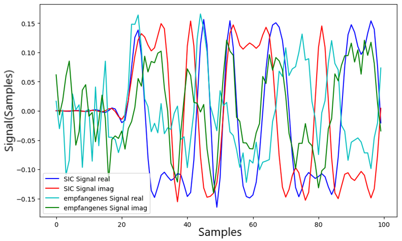
Preparing for SIC

After demodulation comes a critical step: reconstruct the user waveform as it would have looked—ideally—before superposition.

Reconstruction

• Symbols → complex constellation points (including null symbol if used)
• Upsample to the pulse-shaping sample rate
• Convolve with the same pulse as in the transmitter (RRC)

Goal: a clean reference for the decoded strong user in baseband.

Decoded-user reconstruction uses calculated_original_signal (excerpt from BAT_NOMA_Receiver.py):

def calculated_original_signal(estimated_symbol):
    estimated_Signal = np.zeros(len(estimated_symbol[0:464]), dtype='complex_')
    for m in np.arange(len(estimated_symbol[0:464])):
        if estimated_symbol[m] == 0:
            estimated_Signal[m] = np.cdouble(complex(1, 1))
        if estimated_symbol[m] == 1:
            estimated_Signal[m] = np.cdouble(complex(-1, 1))
        if estimated_symbol[m] == 2:
            estimated_Signal[m] = np.cdouble(complex(-1, -1))
        if estimated_symbol[m] == 3:
            estimated_Signal[m] = np.cdouble(complex(1, -1))
    sub_signal = np.zeros(len(estimated_Signal) * 4, dtype=np.complex64)
    j = 0
    while j <= len(sub_signal) - 1:
        if j % 4 == 0:
            sub_signal[j] = estimated_Signal[int(j / 4)]
        else:
            sub_signal[j] = 0
        j = j + 1
    sub_signal = np.convolve(sub_signal, rcos)
    return np.array(sub_signal, dtype=np.cdouble)

Then phase correction with stored PLL reference, moving-average scaling, and subtraction (SIC block in the same file).

Scaling to received amplitude

Reconstruction must match the actual received component in amplitude and phase. If amplitude drifts, a moving average of symbol peaks (or a channel estimate) helps set the scale robustly.

What gets subtracted

For SIC you typically do not subtract on raw ADC samples blindly; you use the post-matched-filter, synchronized chain—there the strong user’s shape aligns best with the decoded symbol stream.

Without that alignment large residuals remain; the second user stays hidden and NOMA fails in practice.

Why all this effort

Without accurate timing, frequency, phase, and amplitude estimates the reconstruction does not match the superposed receive waveform—subtraction is wrong and errors propagate to later SIC stages.

Chapter 5 – Successive interference cancellation (SIC) in detail

Successive interference cancellation (SIC) is the mechanism that makes NOMA practical.

Chapter 4 prepared the processing chain; here the superposed user contributions are actually separated.

Goal: decompose the composite receive signal into its components—or isolate them sequentially enough that weaker users can be demodulated.

Basic principle

For two users in baseband the receive signal can be written as

\[ r(t) = s_1(t) + s_2(t) + n(t) \]

• \(s_1(t)\): dominant user
• \(s_2(t)\): weaker user
• \(n(t)\): noise (and any modeled residual interference)

SIC idea: estimate and demodulate the strong term \(s_1\) → reconstruct → subtract from the receive waveform → \(s_2\) becomes more visible for the next demodulation pass.

Algorithm flow

Step 1 – Detect the dominant layer

After Chapter 4 preprocessing the signal is synchronized, frequency offset is roughly corrected, and after the matched filter you have a suitable waveform for decisions.

The strongest layer can then be demodulated like a single-user link at first.

Note: the weaker user acts like extra noise/interference. BER stays low if the power split and channel quality are right.

Step 2 – Symbol-based reconstruction

Demodulated symbols map to complex constellation points. QPSK example (as built; Gray mapping typical):

• \(00 \rightarrow 1 + j\)
• \(01 \rightarrow -1 + j\)
• \(11 \rightarrow -1 - j\)
• \(10 \rightarrow 1 - j\)

(With the extended alphabet from Chapter 4 a null symbol \((0,0)\) may appear.)

Result: a discrete symbol sequence in I/Q.

Step 3 – Upsampling

The symbol sequence is brought back to the pulse-shaping sample rate: several samples per symbol with (ideally) zeros between—needed to rebuild the continuous transmit pulse.

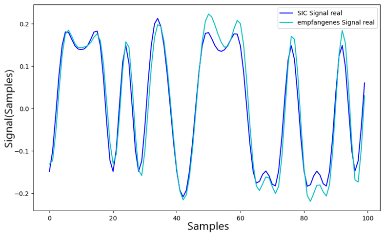
Step 4 – Pulse shaping (reconstruct the transmit waveform)

The upsampled symbol stream is convolved with the pulse shape as in the transmitter:

\[ s_{\mathrm{rek}}(t) = s_{\mathrm{sym}}(t) \ast h(t) \]

Here \(h(t)\) is the root-raised-cosine impulse response (TX side). The result approximates the interference-free transmit waveform of the strong user in baseband—up to scaling and channel phase, aligned in the next step.

Step 5 – Critical: scaling

Practice often departs from naive theory.

Naive (poor): scale only from the raw receive peak—problematic with noise, superposition, and SDR/AGC variation.

Practical: e.g. moving average of symbol peaks (or robust channel amplitude estimate). Benefits: fewer noise outliers, more stable fit under NOMA superposition, tracking over time.

Step 6 – Subtraction

The actual SIC step in baseband:

\[ r_{\mathrm{neu}}(t) = r(t) - \alpha \cdot s_{\mathrm{rek}}(t) \]

\(\alpha\) bundles amplitude and phase alignment (possibly complex, implementation-dependent).

Important: \(r(t)\) here is the preprocessed signal—filtered and synchronized, not the raw ADC stream. Timing and pulse shape then match between receive and reconstruction.

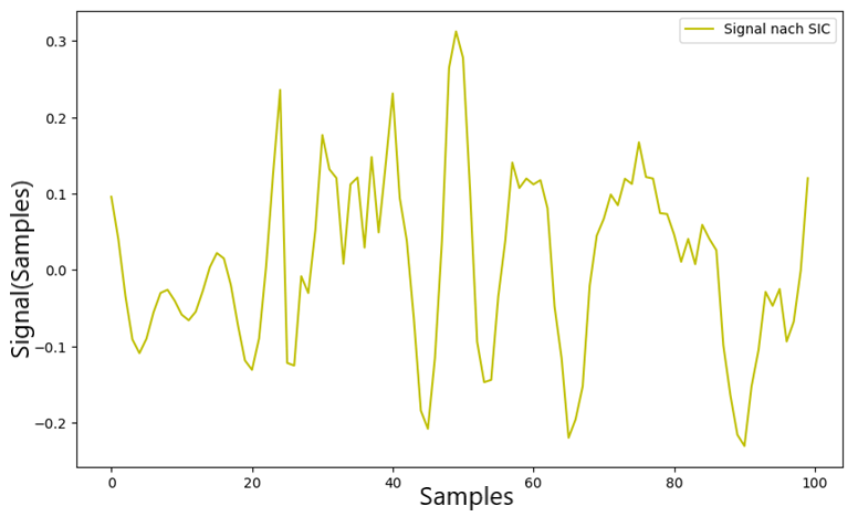
Outcome: the dominant user is largely removed; the weaker user emerges in the residual.

After phase correction of whole_rx, the notebook scales Sic_Signal with a moving average of magnitude peaks and subtracts it from the segment; frequency offset for the second user is corrected next (excerpt from BAT_NOMA_Receiver.py):

Sic_Signal = calculated_original_signal(estsymb)
for o in np.arange(whole_rx.shape[0] - 50 - 48):
    whole_rx[o + 50] *= np.exp(-1j * refph[int(o / 4)])
start_value = (np.mean(np.abs(rx[i0:i0 + 64 * 4:4].real)))
for i in np.arange(0, 1914):
    new_value = (39 * start_value + np.abs(whole_rx[int(i / 4) + 40].real)) / 40
    Sic_Signal[i + 40] = Sic_Signal[i + 40] * start_value * 1.1
    start_value = new_value
rx[i0 - 50:i0 + 464 * 4 + 48] = whole_rx[0:464 * 4 + 50 + 48] - Sic_Signal
rx[i0:i0 + 464 * 4] = rx[i0:i0 + 464 * 4] * np.exp(
    -1j * (-1 * ph0) - 2j * np.pi * ((-1) * f0) / fft_len * np.arange(i0, i0 + 4 * symbols.shape[0]))

i0, ph0, f0, estsymb, refph come from the preamble/PLL chain in the same script.

Error amplification

Subtraction is never perfect. Causes include:

• Noise
• Residual phase and frequency error
• Inaccurate \(\alpha\) or wrong channel estimate
• Sync errors

Residual artifacts can strongly disturb the second user and degrade demodulation after the first SIC stage.

Practical optimizations (engineering notes)

1. Always subtract on the conditioned chain

Subtract on filtered, timing- and frequency-corrected data—not on raw samples. That is often the difference between “SIC works” and “SIC fails.”

2. Phase-locked loop (PLL)

Issue: phase drift → reconstruction no longer matches the receive waveform.

Fix: PLL or equivalent tracking for continuous phase correction—better alignment and much better subtraction over long packets.

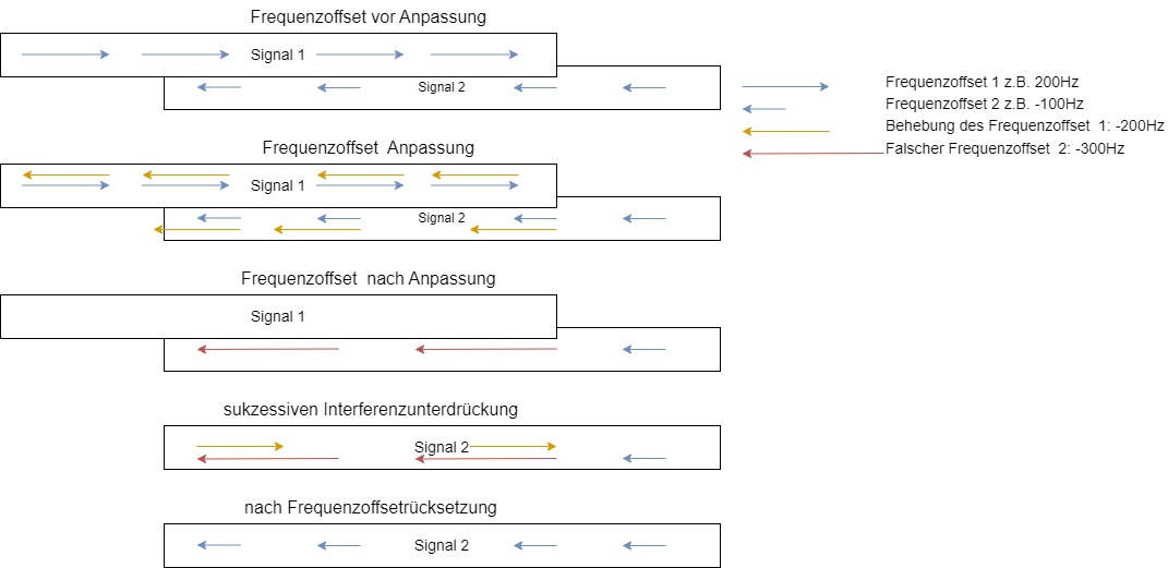
3. Frequency offset with multiple users

Issue: different TX chains can leave different residual offsets; after decoding user 1 the remainder may still be rotated.

Fix: after the first SIC stage re-estimate offset and resynchronize before demodulating user 2.

4. Stitching segments back into the full buffer

If only a time slice is processed, results must be written back consistently—relevant for more than two users or multiple bursts.

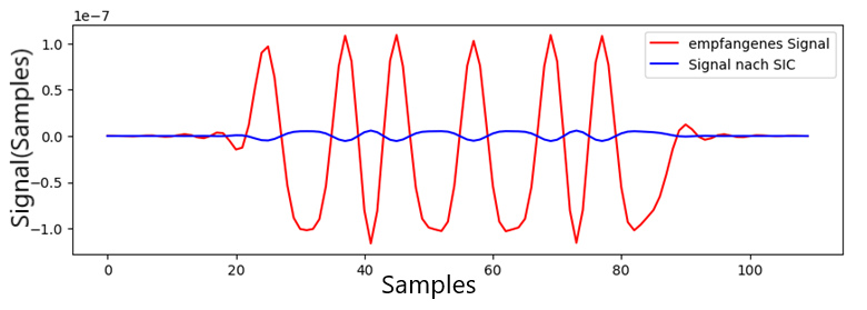
What the optimizations achieved

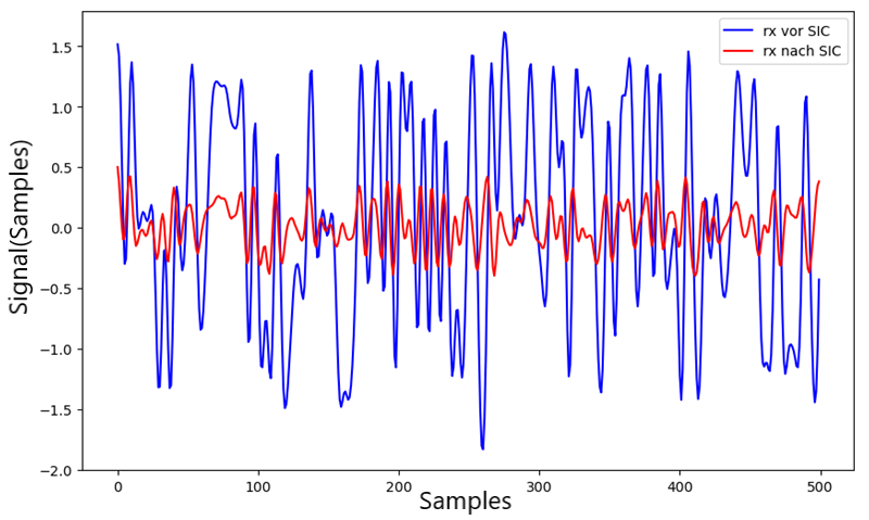
In this setup these steps materially reduced dominant interference (on the order of ~6× measured signal reduction) and improved separation—without them SIC was practically unusable.

The exact factor depends on SNR, power ratio, and implementation; the relative improvement is what matters.

Limits of SIC

SIC is sensitive to:

• Wrong power ratio
• High noise
• Inaccurate synchronization

Critical: if the first user is decoded wrongly, reconstruction is wrong, subtraction harms the residual, and the second user becomes unusable—classic error propagation.

Main takeaway

SIC is not simple “subtract one signal.” It is a precise pipeline of demodulation, reconstruction, amplitude/phase alignment, and subtraction—every error burdens all later stages.

Chapter 6 – Running NOMA on real hardware

After the detailed look at signal processing and SIC, this chapter describes how NOMA was implemented and tested in a concrete lab setup.

Focus: real superposition, detecting both users, applying SIC, and getting a usable decode of the weaker user.

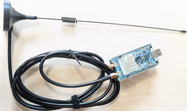
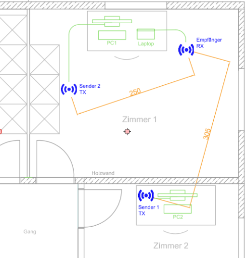
Test setup

The system consists of:

• 2 transmitters (one SDR each)
• 1 receiver (SDR)
• Antennas a few meters apart

Scenario (power domain):

• TX1 → higher transmit power (emulates “farther” / weaker channel)
• TX2 → lower transmit power (closer / stronger path)

Effect: the receiver sees a NOMA-like superposition with different dominance between users.

The photo below shows the bench with antennas and SDR hardware.

Challenge: truly simultaneous transmission

Transmitting two signals at the same time is harder in practice than it sounds.

Control used TCP—small but variable latency. Bursts are very short (order of milliseconds), so even minor jitter matters.

Goal: maximize temporal overlap of both bursts at the receiver despite imperfect triggering.

A small control script (or flowgraph block) sends commands to both TX paths (“send now”) in parallel or sequence. Because of TCP buffering and OS scheduling the absolute timing of the two RF bursts is not deterministic; preamble correlation at the receiver is therefore essential to find each contribution in the mixture—and again for user 2 after SIC.

clientSocket = socket.socket(socket.AF_INET, socket.SOCK_STREAM)
clientSocket2 = socket.socket(socket.AF_INET, socket.SOCK_STREAM)
clientSocket2.connect(("192.168.1.153", 9092))  # second PC
clientSocket.connect(("localhost", 9092))
while i < 1:
    time.sleep(0.2)
    clientSocket2.send(send_zeros)
    clientSocket2.send(frame)
    clientSocket2.send(send_zeros)
    time.sleep(0.01)
    clientSocket.send(send_zeros)
    clientSocket.send(frame)
    clientSocket.send(send_zeros)

Adjust IP/ports to your setup; frame carries payload bytes after adjust_data plus null-symbol fill.

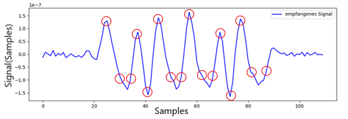
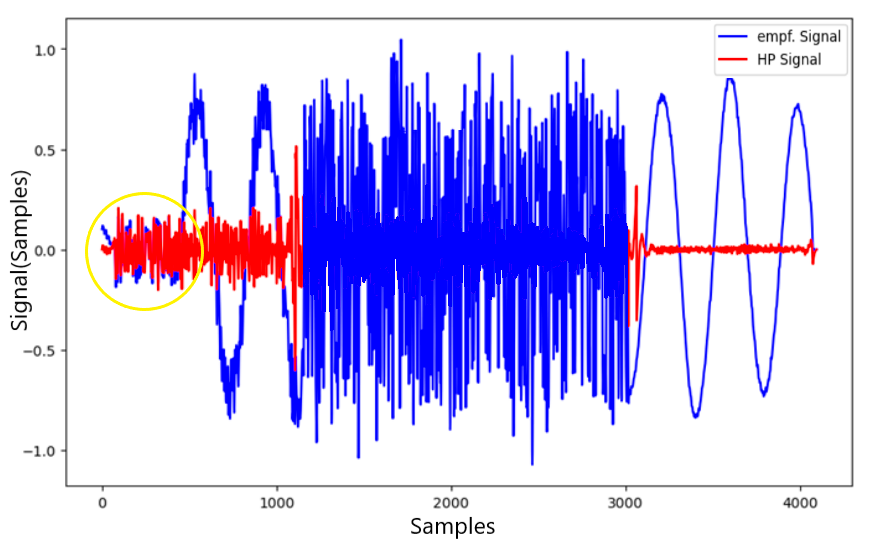
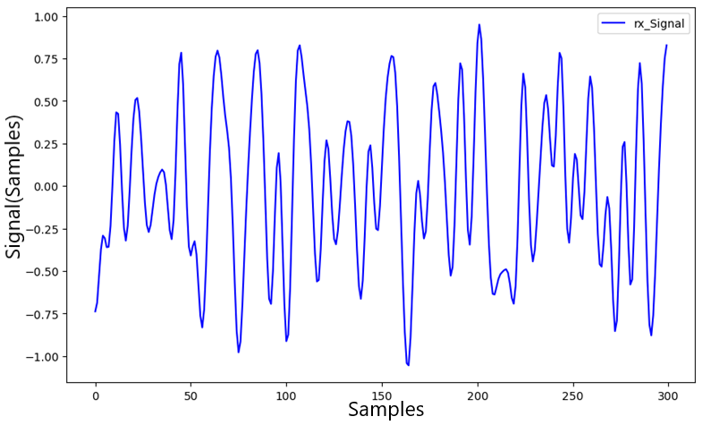
Receiving the superposed signal

The baseband capture shows, as expected:

• no constant envelope,
• visible fluctuations,
• no clean single-user symbol structure in the raw trace.

Interpretation: multiple users superpose—this waveform is the input to preamble search and SIC.

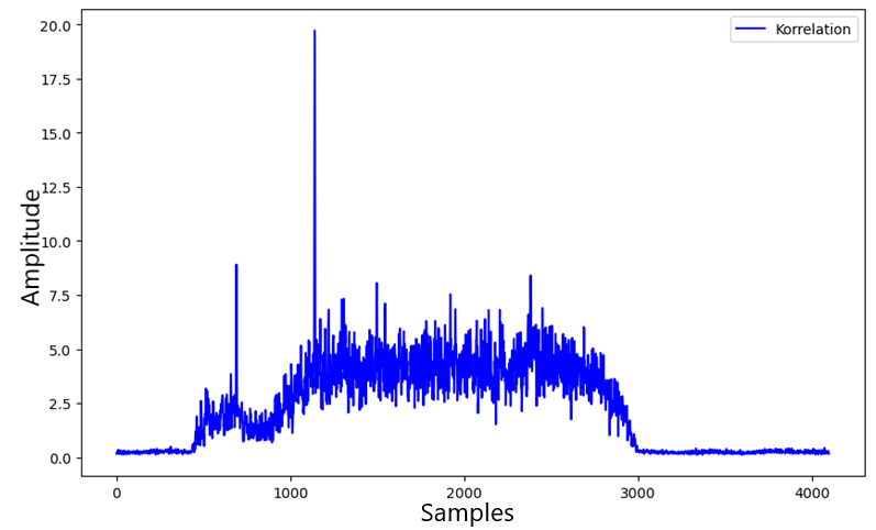
Step 1 – Detect the first signal (preamble)

As in Chapters 4/5: cross-correlate with the known preamble.

Result: a strong peak → start of the first usable segment / evaluated burst.

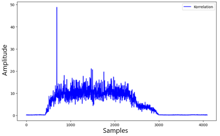
Reading the time trace

Early samples look calmer; later on the trace looks more “torn.”

Interpretation: one user dominates early; overlap with the second user grows later—consistent with offset or overlapping bursts.

Step 2 – Decode the dominant user

The stronger user is demodulated first.

Observations: still decodable despite overlap; symbol phases stay fairly stable.

Estimated BER (order of magnitude): very low, about \(5 \cdot 10^{-3}\) (~0.5% bit errors)—depends on SNR and exact burst alignment.

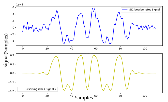
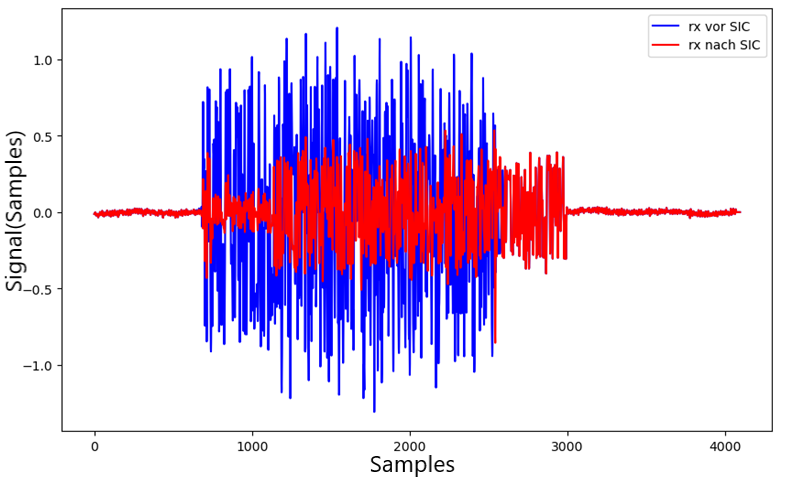
Step 3 – Apply SIC

The dominant contribution is removed with the usual recipe: reconstruct (symbols → pulse), scale, subtract from the conditioned receive buffer.

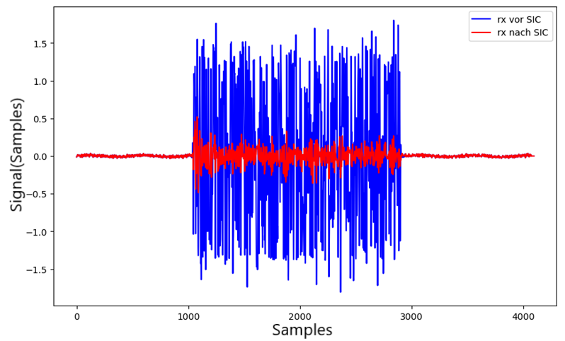
Effect of subtraction

After subtraction the residual amplitude drops and the structure changes.

Crucially: the second user becomes more visible—it had been “hidden” under the dominant layer.

Step 4 – Detect the second signal

Cross-correlate again with the preamble on the residual.

Observation: a new peak appears; user 1’s energy in the residual is much lower.

Conclusion: evidence that the SIC chain works in this setup—user 2 becomes findable again.

Step 5 – Decode the second signal

The weaker user is demodulated.

Observations: more noise, less stable symbol angles than for user 1.

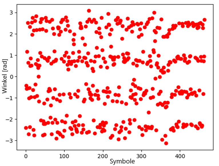
Estimated BER: higher, order \(10^{-2}\) (~1%)—expected from residual interference after SIC and lower effective SNR.

Why the second user is harder

• Residual error from imperfect subtraction
• Non-ideal overlap / timing in the experiment
• Noise hits the weaker layer harder

Typical NOMA behavior: the second stage is always the fragile one.

Overall assessment

• Success: both signals were detected and separated.
• Success: superposition was made practically separable with SIC in this setup.
• Limitation: user 2 quality stays well below user 1—as theory and SIC error propagation predict.

Practical takeaways

1. NOMA works in hardware—not only in simulation; real superposed SDR waveforms could be separated here.
2. Power ratio: too large a gap buries the weak user; too small a gap breaks dominance and hurts the first demodulation.
3. Sync: small timing errors have large impact—especially with short packets.
4. SIC is the bottleneck: subtraction quality largely decides whether user 2 is usable.

Engineering notes

Theory and practice diverge.

Typical real effects in this test:

• Jitter and latency from TCP control
• Unstable amplitudes (AGC, hardware, clipping)
• Never perfectly simultaneous, perfectly overlapping bursts
• Extra hardware imperfections (offset, phase)

That is why filtering, sync, scaling, and PLL in Chapters 4–5 were not optional extras—they were required to make SIC stable.

Chapter 7 – Evaluation and system performance

After running NOMA in the test bench the key question is:

How reliably can signals be separated in practice?

Two quantities matter most:

• Bit error rate (BER)
• Dependence on the user power ratio

BER as the main metric

BER is the fraction of bits received in error:

\[ \mathrm{BER} = \frac{\text{wrong bits}}{\text{total bits}} \]

Lower BER means better decoding under the chosen conditions.

The receiver notebook forms BER from symbol deviations versus reference symbols (excerpt from BAT_NOMA_Receiver.py):

error_sum = 0
for l in np.arange(symbol_len):
    error = ((estsymb[l] - symbols[l] + 8) % 4)
    if error == 3:
        error = 1
    error_sum = error_sum + error
BER = error_sum / (symbol_len * 2)

Bursts with BER below 0.1 count as successfully received (per the evaluation notes).

Results for user 1 (dominant)

The stronger user is decoded directly from the superposed capture.

Observations: very stable symbol decisions; user 2 only moderately interferes; low error rate.

Typical lab values: \(\mathrm{BER} < 0.01\) (under 1%).

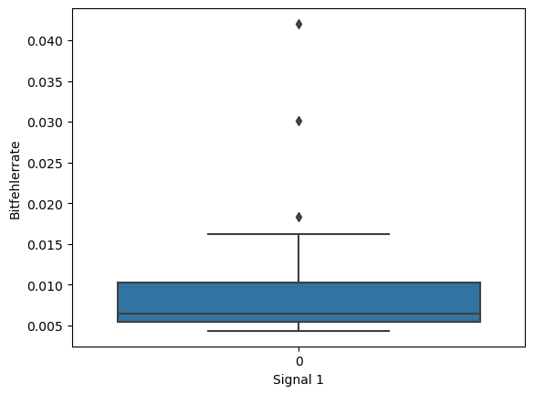
Interpretation (signal 1)

The dominant layer is robust because it carries the largest effective amplitude and user 2 behaves mostly like extra disturbance in the first stage.

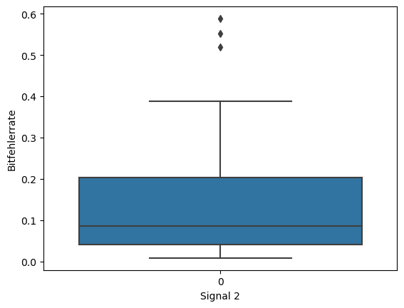
Results for user 2 (after SIC)

The weaker user is evaluated only after subtracting the dominant user.

Observations: much higher spread, more sensitivity to tolerances, stronger dependence on SIC quality and noise.

Typical BER range: roughly \(0.01\) to \(0.1\), strongly tied to power ratio and burst quality.

Why user 2 errs more

• Incomplete or inaccurate SIC
• Residual artifacts from user 1
• Noise
• Residual sync error

This is the main limitation in this build: stage two carries almost all the fragility.

Impact of the power ratio

The main knob in the experiment is the ratio of received powers. With \(P_1\) for the dominant user and \(P_2\) for the weaker user (both measured at the receiver), define

\[ R = \frac{P_2}{P_1} \]

(exact definition follows the lab logging).

What the measurements show

There is a clear optimum: in this run the best \(R\) was roughly \(0.4\)–\(0.5\).

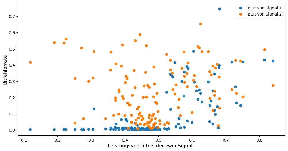
Outside the optimum

• If user 1 is too dominant (\(R\) too small): user 2 is heavily masked and hard to recover after SIC.
• If user 1 is too weak (\(R\) too large): the first demodulation becomes error-prone and the SIC chain collapses—errors propagate.

Interpretation

NOMA here works only in a fairly narrow power window—one of the most important practical lessons.

BER spread

In the favorable \(R\) region:

• Signal 1: very stable, few outliers, consistently decodable.
• Signal 2: wider spread—some bursts much better, others much worse.

Median (signal 2, evaluated dataset): about \(\mathrm{BER} \approx 0.08\).

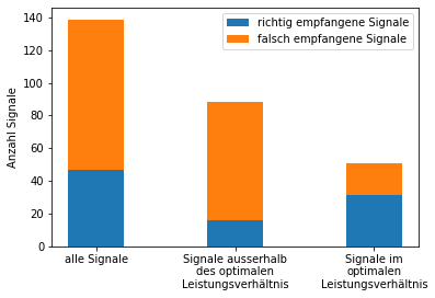
Success rate

A burst was defined as “successfully received” when:

Criterion: \(\mathrm{BER} < 0.1\).

Results (experiment):

• Across all settings: ~34% of cases met the criterion,
• In the optimal power region: ~60%.

Interpretation

The setup behaves like NOMA should, but it is not yet reliable enough for strict IoT targets—highly sensitive to power ratio and signal quality.

Main system limits

1. Unstable power split: SDR/AGC amplitudes drift over time and between bursts.
2. SIC imperfections: subtraction is never perfect; residuals hurt stage two.
3. Noise and channel: affect both users; worse for the weak layer.
4. Sync errors: timing and frequency are never ideal—small offsets, large impact on short packets.

Key takeaways

1. NOMA is parameter-heavy—performance drops fast without a good setup.
2. SIC is the critical step—subtraction quality largely decides success.
3. The second user is always harder—lower effective SNR and more impairment after stage one.

Toward a more robust system

To make similar setups much more reliable, useful additions include:

• Forward error correction (FEC) and optionally interleaving
• Adaptive power or rate control (tuning \(R\) and data rate)
• Better synchronization (tighter triggering, common reference instead of TCP jitter)
• For research rigs: learned or iterative SIC refinements for channel and residual interference

Chapter takeaway

NOMA works in the lab—but it is not plug-and-play.

• Good results are possible in the optimal power region.
• Practical limits show up via SIC residuals, noise, and synchronization.
• Performance depends strongly on system parameters—especially \(P_2/P_1\) and first-stage demodulation quality.

Chapter 8 – Conclusion and outlook

This chapter summarizes the bench results and places them in a technical outlook. Additional plots are omitted here on purpose; the key curves are in Chapter 7.

Summary

The article shows how non-orthogonal multiple access (NOMA) can be implemented with software-defined radio and tested in the lab.

Core idea: several users transmit at the same time in the same band; separation happens in the receiver—mainly via successive interference cancellation (SIC).

What the build confirmed:

• Superposed waveforms can be peeled back into usable single-user streams.
• SIC works on real SDR chains when preprocessing and scaling are right.
• A second, weaker user can be revealed and demodulated after subtracting the dominant user.

Bottom line: NOMA is not only a textbook concept—it can be demonstrated in a controlled setup.

Practice vs. theory

One key lesson: theory sounds easier than the lab.

The NOMA principle is quick to state; the real chain shows:

• Signals are noisy and non-ideal.
• Amplitudes vary (AGC, hardware, clipping).
• Frequency and phase errors are always present.
• Synchronization is never perfect—especially with short bursts and external triggering.

Consequence: SIC only succeeds when filtering, sync, phase, and amplitude processing are tightly matched.

Main technical lessons

1. Power ratio: it decides success—too large a gap hides the weak user; too small a gap breaks dominance and the first detection. There is a narrow optimum (Chapter 7).
2. SIC at the core: subtraction quality decides almost everything; small reconstruction errors strongly affect the second user. SIC is the bottleneck.
3. DSP focus: the hard part is less “RF alone” than the processing after it—filtering, synchronization, phase tracking, and scaling enable NOMA in this form.
4. Weak users: the second signal is disadvantaged physically and algorithmically—more noise, higher sensitivity, harder reconstruction. That is a property of power-domain NOMA with SIC, not merely a coding slip.

Where NOMA can help

Despite the challenges, NOMA has potential for dense future radio deployments:

• IoT: many devices in parallel, often moderate rates, interest in spectrum efficiency.
• Smart cities: sensor fields, traffic and infrastructure data—high device counts, limited resources.
• Low-energy links: less rigid orthogonal assignment can cut overhead—paired with careful power planning and robust receivers.

Possible improvements

To make NOMA more deployment-ready:

1. Adaptive power control: transmitters adjust power so the optimum ratio stays more stable.
2. Machine learning for SIC/channel: neural or iterative estimators for residual interference and channel—more robust to noise and model error (research/prototype stage).
3. FEC: cuts BER on the second user path and greatly softens SIC residuals.
4. Better synchronization: tighter time/frequency lock (common reference, better triggering) → smaller errors before subtraction.

Engineering reflection

In practice the hardest issues are rarely “missing theory” but implementation detail.

Typical invisible effects:

• Small timing slips
• Tiny phase offsets
• Unstable amplitudes
• Non-ideal hardware (offset, drift)

Those details often decide whether a demonstrator works or falls apart.

Closing thought

NOMA underscores that modern wireless is largely algorithms and DSP—not only antennas and amplifiers.

Combining RF, software, and models opens paths to use spectrum more efficiently.

Final note

The described setup ties DSP, over-the-air transmission, and system integration together and shows how concepts become measurable.

That link between theory, implementation, and measurement matters for evolving IoT and communication systems—whether NOMA appears in standards exactly this way or simply as one tool among many.