Designing digital filters – from cutoff frequency to coefficients (IIR / biquad)
How to obtain \(b_0, b_1, b_2, a_1, a_2\) directly from \(f_c\), \(f_s\), and \(Q\) and use them in code
Theory & derivation: Deriving a second-order digital low-pass filter (analog \(G(s)\), bilinear transform, \(H(z)\), and difference equation).
How do you compute digital filters from cutoff frequency and sample rate?
This question is among the most common in signal processing, audio development, and embedded programming.
This article walks step by step through:
- how to compute filter coefficients \(b_0, b_1, b_2, a_1, a_2\) from cutoff \(f_c\), sample rate \(f_s\) (and quality \(Q\))
- and how to use them immediately in the recursion (C, DSP, real time)
Goal: from the desired filter to a finished implementation.
What does “designing digital filters” mean?
A digital filter is not described internally with frequencies, but with a difference equation:
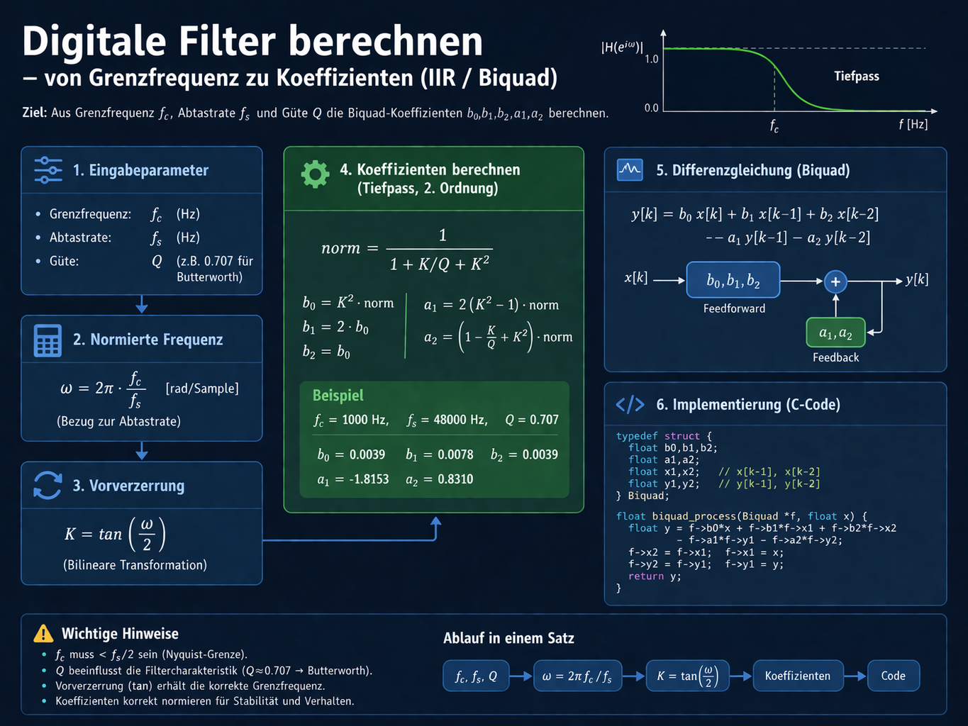
\[ y[k] = b_0 x[k] + b_1 x[k-1] + b_2 x[k-2] - a_1 y[k-1] - a_2 y[k-2] \]
For the filter to exhibit the intended frequency behavior (e.g. low-pass at 1 kHz), \(b_i\) and \(a_i\) must be computed consistently with \(f_c\), \(f_s\), and \(Q\).
Input parameters
For a typical second-order IIR low-pass you need:
- Cutoff frequency \(f_c\) (e.g. 1000 Hz)
- Sample rate \(f_s\) (e.g. 48 000 Hz)
- Quality factor \(Q\) (e.g. \(1/\sqrt{2} \approx 0.707\) for Butterworth)
In practice this is enough for many standard low-passes.
Step 1: Normalized angular frequency
The normalized angular frequency describes how close the cutoff is to half the sample rate. It is the central link between the analog view (Hz) and the digital system (samples).
\[ \omega = 2\pi \frac{f_c}{f_s} \]
Step 2: Bilinear transform (prewarp)
The bilinear transform warps frequencies in a nonlinear way. Without correction, the filter would not operate exactly at the desired cutoff.
Prewarping compensates for this warping. The tangent term ensures the cutoff in the digital filter matches exactly.
\[ K = \tan\left(\frac{\omega}{2}\right) \]
Step 3: Coefficients (second-order low-pass)
The coefficients have a clear structure:
- b0, b1, b2 set the contribution of the input (feedforward)
- a1, a2 set the feedback
A low-pass results because rapid changes (high frequencies) are attenuated through feedback.
\[ \mathrm{norm} = \frac{1}{1 + \frac{K}{Q} + K^2} \]
\[ b_0 = K^2 \cdot \mathrm{norm},\quad b_1 = 2 b_0,\quad b_2 = b_0 \]
\[ a_1 = 2(K^2 - 1)\cdot \mathrm{norm},\quad a_2 = \left(1 - \frac{K}{Q} + K^2\right)\cdot \mathrm{norm} \]
These values can be plugged directly into the recursion (see below).
Example (rounded)
\(f_c = 1000\) Hz, \(f_s = 48\,000\) Hz, \(Q = 0.707\):
- \(b_0 \approx 0.0039\), \(b_1 \approx 0.0078\), \(b_2 \approx 0.0039\)
- \(a_1 \approx -1.8153\), \(a_2 \approx 0.8310\)
This calculator turns a desired cutoff into concrete filter coefficients. That means: you specify which frequencies should pass— and get the numbers your microcontroller or DSP can use directly.
Interactive calculator: digital low-pass (biquad)
Coefficients of a second-order digital IIR low-pass from cutoff frequency, sample rate, and quality \(Q\). Values recompute automatically when inputs change; you can also copy coefficients to the clipboard.
Note: You can paste the coefficients straight into your code. Make sure your filter uses normalized coefficients (a0 = 1).
Python code for the computation
import math

def lowpass(fc, fs, Q=0.707):
    omega = 2 * math.pi * fc / fs
    K = math.tan(omega / 2)

    norm = 1 / (1 + K / Q + K * K)

    b0 = K * K * norm
    b1 = 2 * b0
    b2 = b0

    a1 = 2 * (K * K - 1) * norm
    a2 = (1 - K / Q + K * K) * norm

    return b0, b1, b2, a1, a2
Using the recursion (C / embedded)
y = b0*x + b1*x1 + b2*x2
  - a1*y1 - a2*y2;
This matches the usual pattern on microcontrollers, audio DSPs, and real-time systems (states \(x_1,x_2,y_1,y_2\) as in the low-pass article).
Effect of quality \(Q\)
\(Q\) sets the shape and sharpness of the transfer function:
| \(Q\) | Behavior |
|---|---|
| \(0.5\) | more damped |
| \(0.707\) | Butterworth (common default) |
| \(> 1\) | resonance / peak near \(f_c\) |
Many searches use phrases like “Q factor filter meaning”—that refers exactly to this role of \(Q\) in the design.
Typical mistakes
- Cutoff above the Nyquist limit \(f_s/2\)
- Wrong signs for \(a_1, a_2\) in the implementation (compare with the standard difference equation)
- No frequency prewarping → wrong effective cutoff (addressed here by \(K=\tan(\omega/2)\))
- Very high \(Q\): numerical sensitivity and possible instability with wrong parameters
Why this method is standard
The combination of bilinear transform and biquad structure is widely used because it is stable, efficient, and straightforward to implement. Typical applications: audio equalizers, DSP systems, control, and embedded devices.
Conclusion
With a few parameters you get: cutoff frequency → coefficients → finished recursion. IIR biquad low-passes are therefore among the most important tools in digital signal processing—alongside the theoretical derivation via \(H(z)\).
Author: Ruedi von Kryentech
Created: 6 Apr 2026 · Last updated: 6 Apr 2026
Technical content as of the last update.