Electrical engineering article

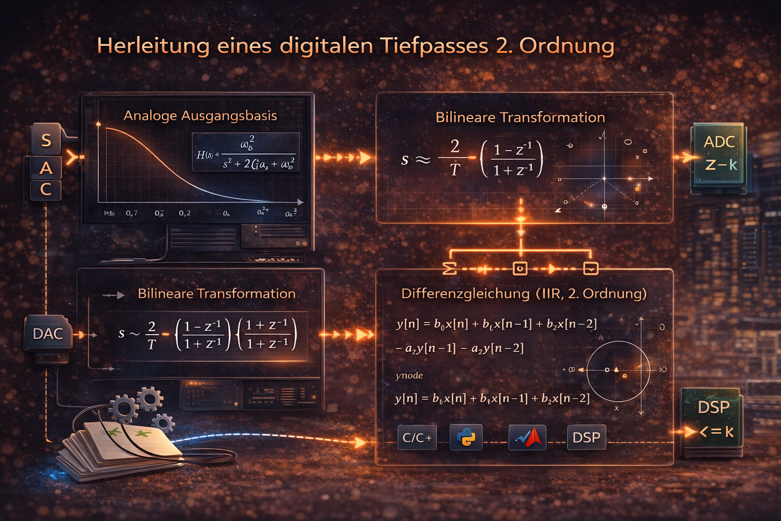
Deriving a second-order digital low-pass filter

From the analog transfer function to discrete-time implementation

Digital filters are central to modern signal processing—from audio to control. A particularly efficient and widely used structure is the second-order IIR filter (biquad).

This article walks step by step from an analog transfer function to a digital filter and how it maps directly to code.

Hands-on: Designing digital filters – biquad coefficients from cutoff and sample rate (with calculator)

What is an IIR filter? (brief)

An IIR (infinite impulse response) filter uses past output samples to compute the current output. That yields strong filtering with little computational cost.

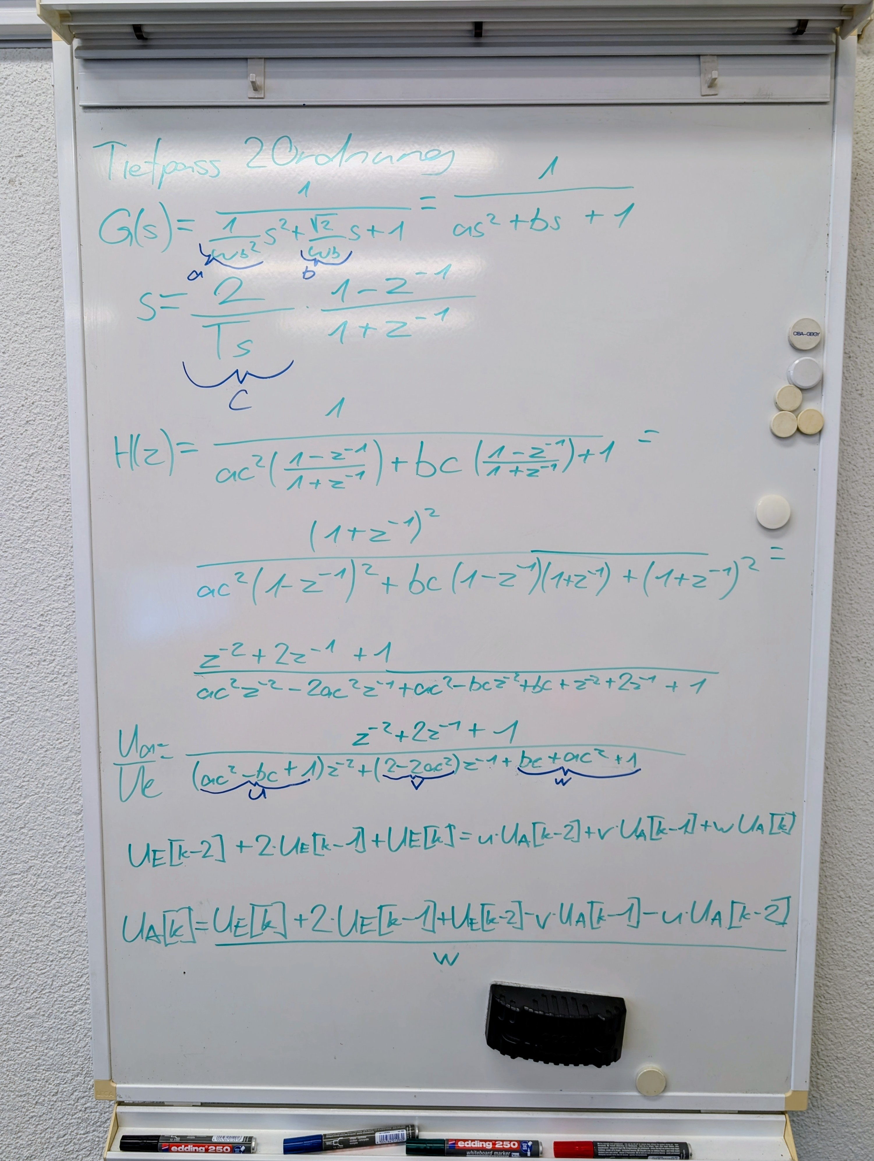
1. Analog starting point

A normalized second-order low-pass is described by:

\[ G(s) = \frac{1}{a s^2 + b s + 1} \]

Here \(a\) mainly sets the cutoff frequency and \(b\) the damping / quality factor.

2. Bilinear transform

For discretization, the bilinear transform is used:

\[ s = \frac{2}{T_s}\cdot\frac{1-z^{-1}}{1+z^{-1}} \]

With \(c = \frac{2}{T_s}\), in the z-domain:

\[ H(z) = \frac{z^{-2} + 2z^{-1} + 1}{(a c^2 - b c + 1) z^{-2} + (2 - 2a c^2) z^{-1} + (b c + a c^2 + 1)} \]

3. Difference equation (IIR, 2nd order)

With input \(U_E[k]\) and output \(U_A[k]\):

\[ U_A[k] = U_E[k] + 2U_E[k-1] + U_E[k-2] - vU_A[k-1] - uU_A[k-2] \]

with:

\[ u = a c^2 - b c + 1,\quad v = 2 - 2a c^2,\quad w = b c + a c^2 + 1 \]

This is a classic biquad IIR. The same structure can be written in standard \(b_0, b_1, b_2\) and \(a_1, a_2\) form after normalization (see below).

From math to code

The difference equation in general form (input \(x[k]\), output \(y[k]\)):

\[ y[k] = b_0 x[k] + b_1 x[k-1] + b_2 x[k-2] - a_1 y[k-1] - a_2 y[k-2] \]

It describes the filter mathematically. For runnable code you map it to memory and processing order.

1. Meaning of the terms

• \(x[k]\) – current input sample
• \(x[k-1]\), \(x[k-2]\) – past input samples
• \(y[k-1]\), \(y[k-2]\) – past output samples

Important: the CPU does not “remember” history by itself—past samples must be stored in variables.

2. Define state (memory)

For history you typically use:

x1 = x[k-1]
x2 = x[k-2]
y1 = y[k-1]
y2 = y[k-2]

These are the filter states.

3. Translate the equation to code

The formula maps almost 1:1:

y = b0 * x
  + b1 * x1
  + b2 * x2
  - a1 * y1
  - a2 * y2;

It is the same difference equation—just in code form.

4. Update state

After computing the output, shift stored values for the next sample:

x2 = x1;
x1 = x;

y2 = y1;
y1 = y;

Thus the current value becomes the “past” value on the next iteration.

5. Per-sample flow

For each new input sample the same cycle runs:

1. read new input \(x[k]\)
2. compute output \(y[k]\)
3. update state

That is what a function like biquad_process() typically does.

6. Intuition

The filter keeps the last values and weights them with coefficients: feedforward via current and past inputs (\(b_0, b_1, b_2\)), feedback via past outputs (\(a_1, a_2\)). That produces the usual filter behavior (e.g. low-pass).

7. Typical mistakes

• not updating state after the output → wrong or unstable behavior
• wrong order when shifting state
• forgetting the sign for \(a_1, a_2\) in code (in standard form they appear subtracted)
• using non-normalized coefficients when the recursion expects normalized form

Equation → code in short: write the formula → store state → compute each sample → shift state. That is the core idea of direct-form II IIR biquads.

Code implementation (2nd-order IIR)

The derived difference equation maps directly to software. A second-order IIR (biquad) needs only a few state variables and is very efficient.

General form and coefficients

\[ y[k] = b_0 x[k] + b_1 x[k-1] + b_2 x[k-2] - a_1 y[k-1] - a_2 y[k-2] \]

• \(b_0, b_1, b_2\) – feedforward (numerator / input path)
• \(a_1, a_2\) – feedback (denominator / recursion; \(a_0\) is usually 1 after normalization)

Example in C (embedded / MCU)

typedef struct {
    float b0, b1, b2;
    float a1, a2;
    float x1, x2;
    float y1, y2;
} Biquad;

float biquad_process(Biquad *f, float x) {
    float y = f->b0 * x
            + f->b1 * f->x1
            + f->b2 * f->x2
            - f->a1 * f->y1
            - f->a2 * f->y2;

    /* update state */
    f->x2 = f->x1;
    f->x1 = x;
    f->y2 = f->y1;
    f->y1 = y;

    return y;
}

Pros: very few operations per sample, predictable runtime—good for real-time DSP and MCUs.

Example in Python (analysis / simulation)

class Biquad:
    def __init__(self, b0, b1, b2, a1, a2):
        self.b0, self.b1, self.b2 = b0, b1, b2
        self.a1, self.a2 = a1, a2
        self.x1 = self.x2 = 0.0
        self.y1 = self.y2 = 0.0

    def process(self, x):
        y = (self.b0 * x +
             self.b1 * self.x1 +
             self.b2 * self.x2 -
             self.a1 * self.y1 -
             self.a2 * self.y2)

        self.x2 = self.x1
        self.x1 = x
        self.y2 = self.y1
        self.y1 = y

        return y

Link to the derivation

The derivation uses analog parameters \(a\), \(b\) in \(G(s)\), \(c = 2/T_s\), and discrete coefficients \(u\), \(v\), \(w\). From that you build \(H(z)\); for implementation, terms are converted to standard biquad form with \(b_0, b_1, b_2, a_1, a_2\), usually by normalizing to the leading denominator coefficient (\(a_0 = 1\)).

Important: the real-time recursion always uses these normalized coefficients.

Practical notes

• Numerics: at high frequencies or low damping, rounding errors matter more.
• Fixed-point vs float: MCUs without an FPU often use fixed-point with scaling.
• Initial values: \(x_1, x_2, y_1, y_2\) usually start at 0 (quiet start).
• Overflow: watch saturation with high gain or integer arithmetic.

Implementation takeaway

A second-order IIR is structurally simple and efficient; the hard part is correct coefficient computation and normalization. Biquads are standard in audio, control, and real-time DSP.

Parameter choice and tools

Continuous analog parameters (\(a\), \(b\) in \(G(s)\)) follow cutoff and damping; \(T_s\) comes from the sample rate. For design, simulation, and verification, Python/NumPy, MATLAB/Simulink, and dedicated DSP tools are common.

Conclusion

The derivation shows how a digital low-pass arises systematically from an analog description. With the biquad structure you get an efficient, practical implementation usable directly in embedded systems, audio, and control.

Correct calculation and normalization of the coefficients is essential—they define the actual frequency response.

More detail in: Computing biquad coefficients from cutoff frequency