Understanding neural networks
Fundamentals, hand calculation, and connection to LLMs
From weights, bias, and activation functions to backpropagation, deep learning, and transformer networks
Summary: This article explains neural networks from the ground up: first with concrete hand calculations and activation functions, then the transition to deep learning, transformers, and LLMs.
Further reading: For architecture details see How does a transformer work? For vector representations of input symbols see Embeddings and vector spaces in neural networks.
1. What is a neural network?
A neural network is a parameterized function \(f_{\theta}\) that maps an input to an output. The parameters \(\theta\) are not set by hand but learned from data.
\[ y = f_{\theta}(x) \]
Historically inspired by biological neurons, technically it is a computing system of weighted sums, nonlinear functions, and many stacked layers.
2. Linear layers, weights, and hand calculation
The elementary building block of many networks is the affine transformation:
\[ z = Wx + b \]
\(W\) is a weight matrix, \(b\) a bias vector. Without nonlinearities the whole network would collapse to a single linear map. Expressive power comes from interaction with activation functions.
In LLMs such matrices appear everywhere: in embeddings, attention projections, feed-forward blocks, and the output projection to the vocabulary.
Computing a single neuron by hand
An artificial neuron first computes a weighted sum of its inputs and adds a bias. That yields a well-defined intermediate value you can compute entirely by hand.
\[ z = w_1x_1 + w_2x_2 + b \]
With \(x_1 = 2\), \(x_2 = 3\), \(w_1 = 0.5\), \(w_2 = -1.0\), and \(b = 0.2\), we get:
\[ z = 0.5 \cdot 2 + (-1.0) \cdot 3 + 0.2 = 1 - 3 + 0.2 = -1.8 \]
This value \(z\) is often called the pre-activation or net input. The activation function then decides how this intermediate value is passed to the next layer.
A small layer with two neurons
A full layer consists of several such neurons sharing the same input but with different weights and biases, producing multiple parallel outputs from one input vector.
For \(x=\begin{bmatrix}1\\2\end{bmatrix}\), \(W=\begin{bmatrix}1.0 & 0.5\\-0.5 & 2.0\end{bmatrix}\) and \(b=\begin{bmatrix}0.1\\-0.2\end{bmatrix}\) we obtain:
\[ z = Wx+b = \begin{bmatrix} 1.0\cdot1 + 0.5\cdot2\\ -0.5\cdot1 + 2.0\cdot2 \end{bmatrix} + \begin{bmatrix} 0.1\\ -0.2 \end{bmatrix} = \begin{bmatrix} 2.1\\ 3.3 \end{bmatrix} \]
This shows the usual matrix notation in compact form. Under the hood it is still the same elementary multiplication, addition, and bias shift.
3. Activation functions with numeric examples
Activation functions provide the nonlinearity needed for rich feature spaces. Classic examples are sigmoid, tanh, or ReLU. Modern transformers often use GELU and SwiGLU.
\[ y = \sigma(Wx+b) \]
For engineers the analogy helps: a linear chain can only model linear systems. Nonlinearity enables saturation, threshold behavior, complex coupling, and high-dimensional approximation.
ReLU as the simplest practical characteristic
ReLU is \(\mathrm{ReLU}(z)=\max(0,z)\) and clips negative values to zero. For our intermediate value \(z=-1.8\), \(\mathrm{ReLU}(-1.8)=0\).
For a positive value like \(z=2.1\) the signal passes through: \(\mathrm{ReLU}(2.1)=2.1\). In engineering terms this is a simple nonlinear characteristic with suppressed negative region.
Sigmoid as a smooth probability map
Sigmoid maps arbitrary inputs to the range \((0,1)\) and suits outputs read as probabilities. Formally:
\[ \sigma(z)=\frac{1}{1+e^{-z}} \]
With \(z=-1.8\), \(\sigma(-1.8)=\frac{1}{1+e^{1.8}}\approx \frac{1}{1+6.05}\approx 0.142\). For \(z=2.1\), \(\sigma(2.1)=\frac{1}{1+e^{-2.1}}\approx \frac{1}{1+0.122}\approx 0.891\).
tanh as a zero-centered activation
\(\tanh(z)\) is similar to sigmoid but outputs values between -1 and 1, centered at zero, so positive and negative activations are represented more symmetrically.
\[ \tanh(z)=\frac{e^z-e^{-z}}{e^z+e^{-z}} \]
For \(z=2.1\), \(\tanh(2.1)\approx 0.97\); for \(z=-1.8\), \(\tanh(-1.8)\approx -0.95\). This shows how tanh compresses large magnitudes into a bounded range without losing sign.
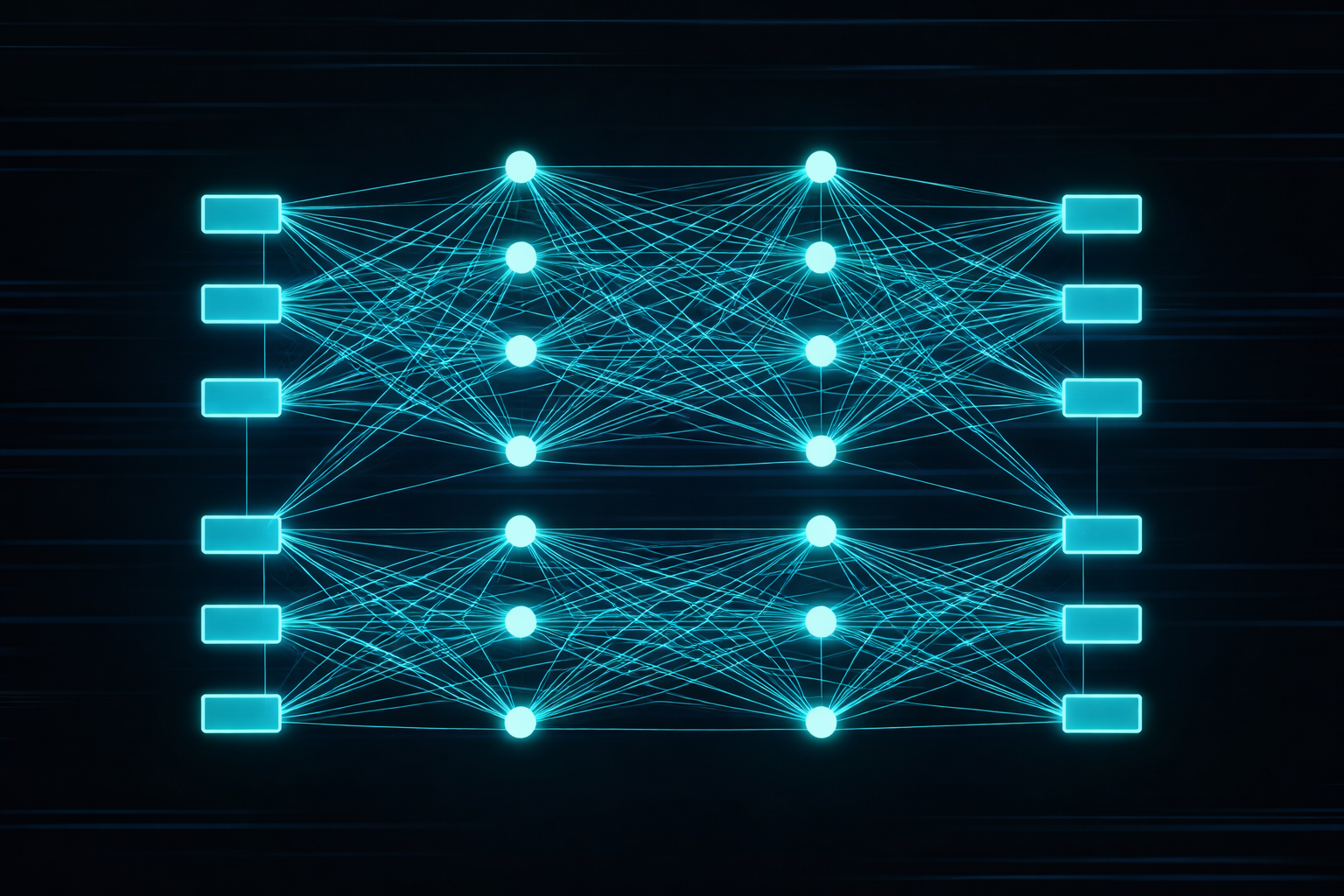
4. Why many layers?
Deep networks learn hierarchical representations. Lower layers capture simple patterns; higher layers capture composed structure. In language processing you can think of it as:
- lower layers: local token patterns and syntax,
- middle layers: relations and structure,
- upper layers: more abstract semantic or task-specific features.
That is why LLMs are called deep learning: performance comes not from a single layer but from many stacked transformations.
5. Backpropagation and learning
The network is trained by computing an error between prediction and target and propagating it backward through the chain rule.
\[ \frac{\partial L}{\partial \theta} \]
These gradients indicate how parameters should change to reduce the error. Without backpropagation, training networks of today’s size would be impractical.
Technically each layer provides not only a forward map but also a contribution to error flow. The chain rule connects all partial terms. That is why clean gradient flow, residual connections, and normalization matter so much in deep networks.
6. Optimization in practice
Plain gradient descent would be:
\[ \theta_{t+1} = \theta_t - \eta \nabla_{\theta}L \]
LLMs typically use Adam or AdamW, plus warmup, learning-rate schedules, mixed precision, gradient clipping, and distributed training. The network is not only a mathematical object but a complex optimization problem.
From an engineering perspective this resembles identifying a strongly nonlinear system under resource limits. Numerics, stability, and hardware—not only the model—strongly affect the outcome.
7. Representation learning instead of hand engineering
A central difference from many classical ML pipelines is that neural networks learn their own features. Instead of hand-crafted feature vectors, useful representations emerge from optimizing the objective.
For LLMs that means: not only output weights but embeddings, internal states, attention projections, and semantic structure are learned jointly. That is a major reason modern language models are more flexible than classical NLP pipelines.
8. How this becomes an LLM
In an LLM the input is a token sequence. Tokens become vectors, pass through many transformer layers, and are finally projected to the vocabulary. The typical objective is:
\[ P(x_t \mid x_1, \ldots, x_{t-1}) \]
An LLM is thus a deep neural network with a specific job: model language structure so the next token can be predicted as accurately as possible.
9. Transformers as a specific architecture
The transformer is the concrete architecture powering modern LLMs. It combines:
- embeddings as input representation,
- self-attention for context-dependent coupling,
- feed-forward networks for nonlinear feature extraction,
- residual connections and layer normalization for stability.
Important: an LLM is not merely “statistics over text” but concretely a large transformer network with billions of parameters.
This is where specialized articles branch off: architecture is covered in detail in How does a transformer work?, while input representation and semantic geometry are deepened in Embeddings and vector spaces in neural networks.
10. Link to electrical engineering
Engineering view: Neural networks read naturally as parameterized multistage signal-processing systems.
Each layer maps an input vector to an output vector. A network resembles a signal chain with linear blocks, nonlinear elements, gain, normalization, and feedback through the optimization process.
Topics like state space, approximation, system identification, stability, and hardware acceleration are familiar to electrical engineers. The main differences are data volume, scale, and high-dimensional feature spaces.
11. Conclusion
To understand LLMs you must understand neural networks. A language model is not a detached AI concept but a deep network whose weights were optimized on huge text corpora.
Transformers, attention, embeddings, and output logits are different building blocks of the same principle: a trained neural network approximates a complex function over language.
If you can hand-compute one neuron, the matrix math of a small layer, and the effect of ReLU, sigmoid, or tanh, you already have the foundation for all later special topics.
For practical next steps see How does a transformer work? and Embeddings and vector spaces in neural networks.
Author: Ruedi von Kryentech
Created: 14 Apr 2026 · Last updated: 14 Apr 2026
Technical content as of the last update.