How does a transformer work?
In-depth technical article on self-attention, QKV, multi-head, LayerNorm, and causal masking
Summary: A transformer is a deep neural network that does not process sequences only step by step but models global contextual relationships between all tokens via self-attention.
Further reading: For neural-network basics see Neural networks behind LLMs. For token input representations see Embeddings and vector spaces in neural networks.
1. Why transformers?
Before the transformer, language processing was dominated mainly by recurrent networks such as LSTM or GRU. These models process text strictly sequentially. That is intuitive but unfavorable for long-range dependencies: information from distant positions must be carried across many time steps.
The transformer fixes this by letting every token access other tokens directly. That makes modeling global relationships much easier. The architecture also maps well to parallel GPU computation.
\[ y = f_{\theta}(x_1, x_2, \ldots, x_n) \]
Crucially: the function is no longer reconstructed only locally via neighborhood or time, but globally via a learnable weighting system between all positions.
2. Difference from a classical neural network
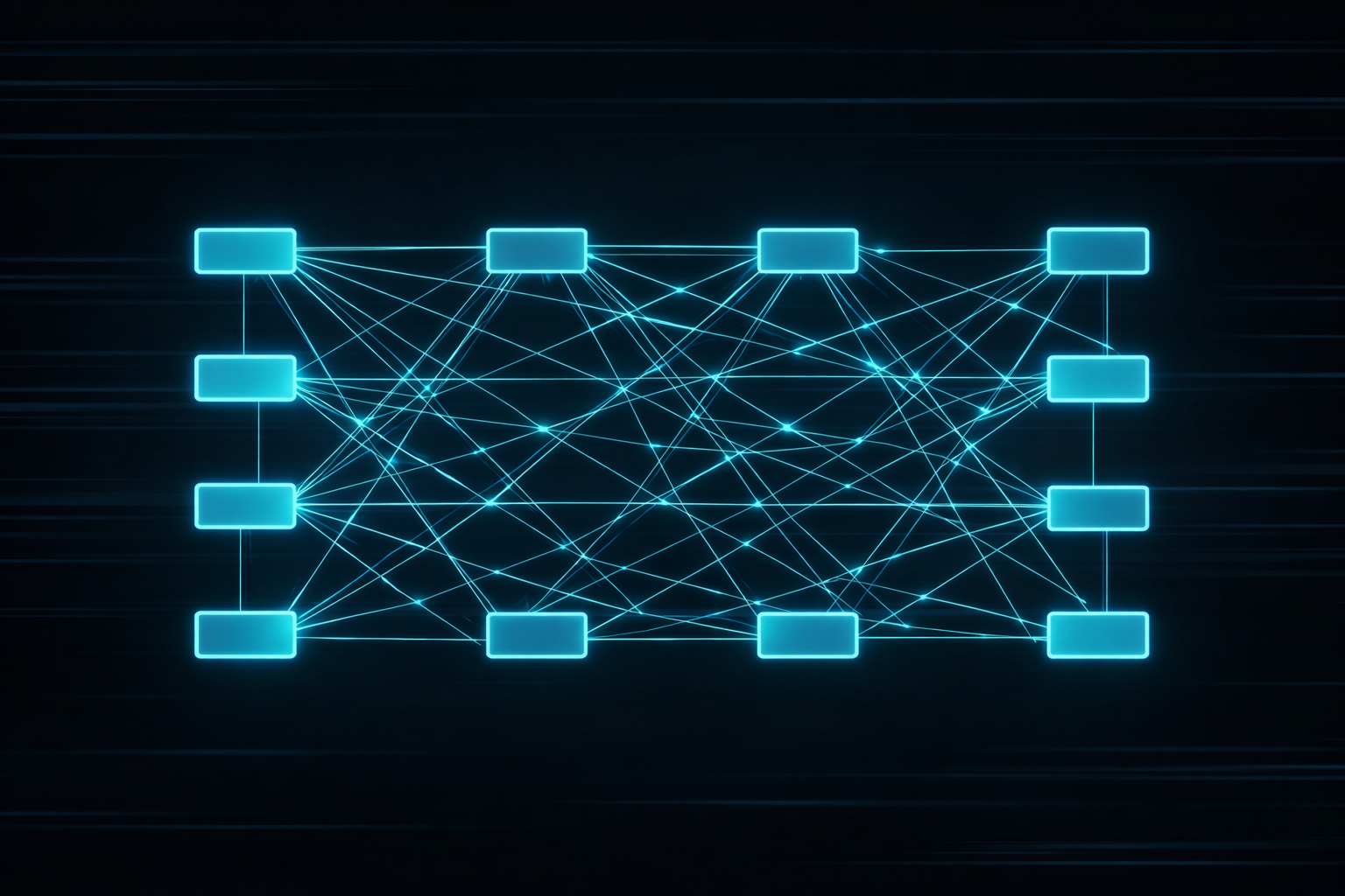
A “classical” neural network usually processes an input layer by layer through fixed weight matrices. The connectivity pattern is predetermined: each layer sees only the previous layer’s output, not dynamically the full context of a sequence.
A transformer is still a neural network, but it extends this idea with self-attention. Connection weights between token positions are not fixed statically but computed from the data itself. That is the central difference.
Classical example: feed-forward network
A simple neural network with one linear layer and activation might compute:
\[ y = \sigma(Wx+b) \]
Take \(x=\begin{bmatrix}1\\2\end{bmatrix}\), \(W=\begin{bmatrix}0.5 & 1.0\\-1.0 & 2.0\end{bmatrix}\) and \(b=\begin{bmatrix}0\\1\end{bmatrix}\). Then first
\[ Wx+b= \begin{bmatrix} 0.5\cdot1 + 1.0\cdot2\\ -1.0\cdot1 + 2.0\cdot2 \end{bmatrix} + \begin{bmatrix} 0\\1 \end{bmatrix} = \begin{bmatrix} 2.5\\4 \end{bmatrix} \]
Then an activation is applied. Important: the weights in \(W\) are fixed for all inputs. The network always responds with the same connectivity structure.
Transformer example: adaptive weighting
A transformer works differently. For a position \(i\) it applies not only a fixed matrix but dynamically weights the importance of other positions:
\[ y_i=\sum_j w_{ij}x_j \]
Suppose three tokens had weights \(w_{i1}=0.1\), \(w_{i2}=0.7\), \(w_{i3}=0.2\). Then token 2 contributes much more to the result than token 1 or 3. In another sentence these weights could look completely different.
That is what makes transformers powerful: they use not only learned static parameters but also context-dependent adaptive couplings between positions.
Practical difference at a glance
| Aspect | Classical neural network | Transformer |
|---|---|---|
| Connectivity | fixed via weights \(W\) | dynamic via attention weights |
| Context | indirect and local | directly global over all positions |
| Language modeling | more limited | much stronger on long dependencies |
A transformer is therefore not the opposite of a neural network but a particularly capable special form of a neural network for sequences and language.
3. Overall signal pipeline
A language transformer can be described roughly as:
Text → tokenization → embeddings → positional info → transformer blocks → logits → probabilities
Each block transforms the current representation into a richer one. At the end stands a distribution over the next token. In an LLM this computation is repeated autoregressively.
From a systems perspective this is a stacked chain of state maps. Each stage takes a vector-space state and produces a new state with higher semantic density. The transformer is therefore not just a “language trick” but structured signal processing on high-dimensional representations.
| Stage | Technical role |
|---|---|
| Tokenization | Split text into discrete symbols |
| Embeddings | Map tokens to continuous vectors |
| Attention | Dynamic weighting of other token positions |
| FFN | Nonlinear feature processing per position |
| Output head | Projection to the vocabulary |
4. Self-attention at the core
Self-attention answers for each token: Which other positions matter for my current interpretation? The mechanism is dynamic and data-driven. The same architecture can weight dependencies very differently per sentence.
Example: in “The sensor reports an error because it is clipping,” the model must resolve what “it” refers to. This is where attention shines.
5. Q, K, V mathematically
From the input matrix \(X\) three projections are formed:
\[ Q = XW_Q,\qquad K = XW_K,\qquad V = XW_V \]
\(Q\) is each position’s query, \(K\) describes what features other positions offer, and \(V\) is the information actually transported.
The attention computation is:
\[ \mathrm{Attention}(Q,K,V)=\mathrm{softmax}\left(\frac{QK^T}{\sqrt{d_k}}\right)V \]
The product \(QK^T\) measures similarity. Division by \(\sqrt{d_k}\) stabilizes value ranges so softmax does not saturate too quickly. The result is a weighted average of value vectors.
6. Multi-head attention
A single attention head can only capture one projection of context. Therefore the mechanism runs in parallel multiple times:
\[ \mathrm{MultiHead}(X)=\mathrm{Concat}(\mathrm{head}_1,\ldots,\mathrm{head}_h)W_O \]
Each head can learn different patterns: syntax, coreference, local neighborhoods, global topics, positional relations, or numeric structure. That yields a richer representation.
Important: heads are not hand-specialized; they emerge from training. Some heads behave almost like neighborhood detectors, others like global channels for topic, sentence references, or positional relations. In large models this yields functional division of labor.
7. Masking in language models
In generative language models a token must not look into the future. A causal mask is used. It sets disallowed connections in the attention score to \(-\infty\) before softmax so those positions receive weight exactly zero after softmax.
That forces position \(t\) to access only positions \(\le t\). Without this constraint the model could “copy” information from the future during training.
8. Feed-forward, residuals, LayerNorm
After attention comes a position-wise feed-forward network:
\[ \mathrm{FFN}(x)=W_2\,\sigma(W_1x+b_1)+b_2 \]
This subnetwork acts like nonlinear feature extraction per token. Modern models often use GELU or SwiGLU.
Residual connections help gradient flow:
\[ y=x+f(x) \]
LayerNorm stabilizes activations via normalization and learnable scaling:
\[ \mathrm{LayerNorm}(x)=\gamma\cdot\frac{x-\mu}{\sqrt{\sigma^2+\varepsilon}}+\beta \]
Here \(\gamma\) and \(\beta\) are learnable parameters, \(\varepsilon\) a small stability term. Together these building blocks keep very deep networks trainable.
From an engineering perspective the attention part is adaptive coupling between positions, while the FFN handles local nonlinear processing within a position. Only both blocks together yield a model that masters both global dependencies and per-position feature refinement.
9. Positional information
Attention alone is permutation-invariant: without extra information the model would not know front from back. Therefore a positional signal is added or rotated into the token representation.
\[ z_i=e_i+p_i \]
Common methods are sinusoidal encodings, RoPE, or ALiBi. From a systems view this explicitly encodes order in state space.
10. Complexity and scaling
Standard attention costs roughly \(\mathcal{O}(n^2)\) in sequence length \(n\) because every position is compared with every other. That is a real bottleneck for long contexts.
Hence many optimizations: FlashAttention, KV cache for inference, sparse attention, segmentation, or hybrid architectures. The transformer is therefore not only a model but a heavily optimized computing system.
For real applications this is central: the theoretically elegant architecture quickly hits hard limits of memory bandwidth, interconnects, and power. Transformer design is always co-design of algorithm and hardware.
11. View from electrical engineering
Engineering view: A transformer reads naturally as an adaptive multistage signal-processing system.
Attention resembles a data-dependent filter:
\[ y_i=\sum_j w_{ij}x_j \]
Unlike classical FIR filters the coefficients \(w_{ij}\) are not fixed but computed from the signal itself. The system becomes adaptive and context-dependent.
Concepts like state space, linear projection, stabilization via normalization, parallelization, and memory bandwidth are familiar from signal processing, control, and hardware acceleration.
12. Conclusion
A transformer is a deep neural network that models language via global, adaptive context weighting. Its strength comes from combining self-attention, multi-head parallelism, feed-forward processing, residuals, LayerNorm, and efficient GPU computation.
This architecture is the technical heart of modern LLMs. To understand how ChatGPT-like systems work, you must understand the transformer.
To deepen the mathematical backbone read next Neural networks behind LLMs. If you care mainly about token input representations, see Embeddings and vector spaces in neural networks.
Author: Ruedi von Kryentech
Created: 14 Apr 2026 · Last updated: 14 Apr 2026
Technical content as of the last update.