How does ChatGPT work?
Large language models—plain language & deep technical analysis
ChatGPT, GPT-4, Gemini, and other LLMs—from the next token to the transformer: concise context and technical foundations
1. What is a large language model (LLM)?
In short: An LLM is a large deep neural network that learns token probabilities from context and generates text from them.
A large language model (LLM) is a mathematical model specialized in processing and generating language. At its core it is not “understanding” in the human sense, but a probability model over text.
Concretely: an LLM computes, for every possible next word (or more precisely: token), the probability that it best fits the text so far.
LLM = deep neural network
Importantly: an LLM is not something totally different from a neural network—it is a large deep neural network. “Deep” means many layers are stacked in sequence that transform the input text step by step.
Modern LLMs are almost always based on the transformer architecture. It consists of repeated blocks of attention, feed-forward networks, residual connections, and layer normalization. The weights of these blocks are adjusted during training so that predicting the next token keeps improving.
What does “neural network” mean here?
A neural network is essentially a large function with many trainable parameters. From an input signal \(x\), many weighted transformations produce an output \(y\):
\[ y = f_{\theta}(x) \]
For an LLM the input is not an image or a sensor reading but a sequence of tokens. The network first maps tokens to vectors and then processes them through many layers until a probability distribution over the next token appears at the end.
Why “deep learning”?
A small network with only one or two layers cannot capture the complexity of natural language well. Many layers yield hierarchical features:
- lower layers capture local patterns and syntax,
- middle layers learn relations and structure,
- deeper layers encode more abstract semantic information.
That is why LLMs clearly belong to deep learning.
Further reading: Neural networks behind LLMs
Language as a mathematical problem
A sentence like “The weather is very … today” is not interpreted as “meaning” internally, but as a sequence of symbols.
The model’s task: Which token comes next with highest probability?
Mathematically this rests on the chain rule for probabilities:
\[ P(x_1, x_2, ..., x_n) = \prod_{t=1}^{n} P(x_t \mid x_1, ..., x_{t-1}) \]
So the probability of an entire sentence is built from the probabilities of each next token, each conditioned on the context so far.
Autoregressive principle (the core of ChatGPT)
An LLM works autoregressively. That means:
- It receives a starting text (prompt).
- It computes probabilities for the next token.
- It selects a token.
- That token is appended to the context.
- The process repeats.
Step by step, a full text is produced.
Important: The model does not know the “full sentence” in advance—it generates it token by token.
What are tokens?
A token is the smallest unit an LLM works with. It can be:
- a whole word,
- a subword (e.g. “ing”, “tion”),
- or even individual characters.
Example: “unbelievable” may split into “un”, “believ”, “able”.
This split is called tokenization and is crucial for model efficiency.
Why this works
Training on huge text corpora lets the model learn, among other things:
- grammar and sentence structure,
- typical word combinations,
- logical relations,
- stylistic patterns.
Even without “real meaning” it can therefore write surprisingly well, answer questions, generate code, and explain complex topics.
Key takeaway: An LLM does not truly understand like a human, does not deliberate, and has no knowledge in the classical sense. It is a very capable statistical pattern matcher.
2. Core mechanism: next-token prediction
Core idea: An LLM generates text autoregressively by repeatedly sampling the next token from a probability distribution.
At each step the model computes a probability distribution over the next token. Formally:
P(t_{k+1} \mid t_1, t_2, ..., t_k)
The chosen token is appended to the context, then the next step follows. This recursive generation turns local decisions into coherent text.
Autoregressive flow in practice
This flow is the operational core of every LLM response. Many local steps combine into globally coherent text.
- A prompt seeds the context,
- the model computes logits for the next token,
- softmax yields probabilities,
- a token is chosen (e.g. greedy or sampling),
- the token is appended and the process repeats.
This loop runs dozens or hundreds of times depending on answer length. Quality depends on both the model and the sampling strategy.
Small intuition example
Context: “The weather is … today”
Possible next tokens might get probabilities like 0.42 (“sunny”), 0.25 (“cold”), 0.11 (“rainy”), and so on.
The model does not “know” the full sentence in advance—it decides step by step.
Why this works well
- local predictions chain into globally coherent text,
- the full context so far enters every step,
- the procedure scales well to large models and datasets.
3. Embeddings & vector spaces—how an LLM represents meaning
Core idea: An LLM does not process words directly, but vectors in a high-dimensional space.
After tokenization each token is mapped to a vector via an embedding matrix. Only then can a neural network process language mathematically.
\[ e_i = E[x_i], \qquad E \in \mathbb{R}^{V \times d} \]
In this space semantic relations become geometric: similar terms lie closer together, dissimilar ones farther apart. In modern LLMs these representations are also context-dependent—the same word can receive different internal vectors depending on the sentence.
Embeddings therefore underpin attention, context modeling, and all further processing in the transformer.
Further reading: Embeddings and vector spaces in neural networks
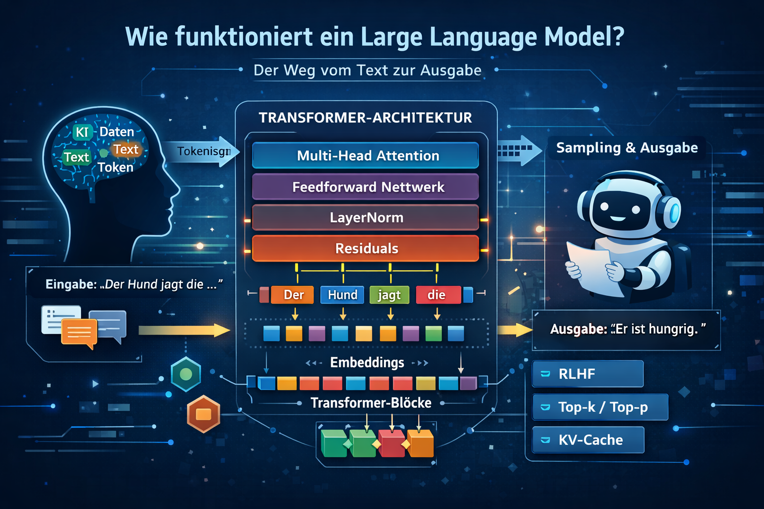
4. Transformer architecture—the heart of an LLM
Why this chapter matters: The transformer is the main reason modern LLMs are so capable.
Almost all modern large language models—including ChatGPT—are based on the transformer architecture. Introduced in 2017, it reshaped NLP.
Technically the transformer itself is a neural network: many trainable weight matrices, nonlinear transforms, and stacked layers. When people say an LLM is a neural network, they usually mean a very large transformer network for language.
A transformer block combines four core elements:
- self-attention for global context coupling,
- feed-forward networks for nonlinear feature processing,
- residual connections for stable gradient flow,
- layer normalization to stabilize activations.
The mathematical core of attention is:
\[ \mathrm{Attention}(Q,K,V)=\mathrm{softmax}\left(\frac{QK^T}{\sqrt{d_k}}\right)V \]
Each token can dynamically weight which other positions in the context matter. Multi-head attention adds parallel perspectives, and a causal mask ensures a language model cannot look into the future.
This architecture is what makes LLMs powerful: global dependencies, parallel computation, and good scalability to very large models.
Further reading: How does a transformer work?
5. Numerical stability & training tricks in LLMs
Key point: LLM training is not only optimization but also a numerical stability problem.
Training a large language model is not only a mathematical problem but a numerical stability problem. Without special techniques training often diverges, produces NaNs, or fails to converge cleanly.
Problem: extreme value ranges
During training very large and very small values appear at once (overflow/underflow).
\[ e^{100} \gg e^{-100} \]
That leads to unstable softmax and unusable gradients.
Log-sum-exp trick (central)
Softmax is computed in a numerically stable way as:
\[ \mathrm{softmax}(z_i)=\frac{e^{z_i-\max(z)}}{\sum_j e^{z_j-\max(z)}} \]
Effect: overflow is avoided; relative probabilities stay the same.
Softmax saturation and attention scaling
If one logit dominates (\(z_i \gg z_j\)), the distribution becomes almost one-hot and the gradient shrinks.
In attention, scaling helps:
\[ \frac{QK^T}{\sqrt{d_k}} \]
It prevents overly large dot products and keeps softmax in a learnable range.
Mixed-precision training
Modern LLMs often use FP16/BF16 for speed and FP32 for critical stable steps.
Because FP16 has less dynamic range, loss scaling is common:
\[ g' = g \cdot S,\qquad g=\frac{g'}{S} \]
This reduces underflow and stabilizes training.
Gradient clipping
With exploding gradients (\(\lVert g\rVert \to \infty\)) updates become unstable. Clipping bounds the norm:
\[ g=\frac{g}{\lVert g\rVert}\cdot c \]
Typically \(c=1.0\).
Layer normalization and residuals
LayerNorm stabilizes activations in the block:
\[ \mathrm{LayerNorm}(x)=\frac{x-\mu}{\sigma} \]
Residuals improve gradient flow:
\[ y=x+f(x) \]
Both are essential for deep transformer networks.
Activation functions and trade-offs
GELU and SwiGLU often yield smoother gradients and better convergence than simpler alternatives.
Techniques like activation checkpointing or ZeRO/FSDP save memory but increase compute and debugging complexity.
NaN issues in practice
Typical causes: learning rate too high, poor initialization, softmax overflow, or FP16 effects.
Practical debugging: check gradient norms, monitor loss, log activation/logit ranges.
PyTorch in practice—numerically stable LLM code
Most modern LLMs are implemented in frameworks like PyTorch. Many stability mechanisms are built in.
Stable cross-entropy
Instead of manual softmax + log, use:
import torch.nn.functional as F

loss = F.cross_entropy(logits, targets)
Internally this uses numerically stable steps such as log_softmax (with log-sum-exp) and negative log-likelihood.
That is more stable and usually faster (fused kernels).
Mixed precision with AMP
from torch.cuda.amp import autocast, GradScaler

scaler = GradScaler()

with autocast():
    logits = model(x)
    loss = F.cross_entropy(logits, y)

scaler.scale(loss).backward()
scaler.step(optimizer)
scaler.update()
FP16/BF16 and FP32 are combined automatically, including loss scaling for stable gradients.
In practice this cuts runtime and memory substantially while keeping numerical stability far better than naive FP16.
Gradient clipping in the framework
torch.nn.utils.clip_grad_norm_(model.parameters(), max_norm=1.0)This limits exploding gradients and prevents unstable updates.
For deep nets and large batches this is an important safeguard. Without clipping, outliers can ruin an entire optimization step.
Typical best practices
Production-style training pipelines often use a few combinations that prove especially robust, addressing optimization, stability, and efficiency together.
- AdamW as optimizer,
- AMP enabled,
- gradient clipping on,
F.cross_entropyinstead of hand-rolled softmax.
This combination matches the industry norm in many LLM training stacks.
PyTorch takeaway
PyTorch hides many complex details behind a few lines of code. Still, understanding numerical stability is essential to debug failures, tune training, and run large models reliably.
Chapter takeaway
Numerical stability is not a detail—it is a prerequisite for trainable LLMs at this scale. Only the combination of stable softmax, scaling, clipping, layer norm, and residuals enables robust training runs.
6. Distributed training & system design for LLMs
Key point: Models of this size are only feasible with distributed training and efficient system design.
A modern large language model cannot be trained on a single machine. Billions of parameters, huge data volume, and very high memory for parameters, gradients, and optimizer states make that impossible.
Core idea: parallelization
To spread load, training is split across many GPUs. The main strategies are:
Without such splitting both runtime and memory would quickly become impractical. Parallelization is not an optional tweak but a prerequisite of modern LLM development.
Data parallelism
Each GPU holds a full model copy and processes different batches.
After each step gradients are averaged:
\[ g=\frac{1}{N}\sum_{i=1}^{N} g_i \]
This is simple and widespread, but only works if the full model fits on one GPU.
Model parallelism
Here the model itself is split, e.g. via:
- tensor parallelism (splitting within layers),
- pipeline parallelism (splitting across layers).
Required for very large models, but it increases communication cost.
Memory optimization (ZeRO / FSDP)
Instead of full replicas, parameters, gradients, and optimizer states are sharded across GPUs. That cuts memory sharply and enables extremely large models.
Central bottleneck: communication
In large clusters raw compute is often not the limit—data exchange between GPUs is. Efficient synchronization and network topology therefore drive overall efficiency.
Real training systems
Modern LLMs run on clusters with hundreds to thousands of GPUs, high-speed networks, and distributed storage. Training becomes a joint effort of software, hardware, and networking.
Impact on the GPU market
High compute demand feeds directly into the real economy:
- strong demand from AI training,
- limited manufacturing capacity,
- focus on data centers rather than consumer hardware.
Effects include rising GPU prices, longer lead times, and high barriers to entry for AI development.
Chapter takeaway
Distributed training is a prerequisite for modern LLMs. It shows clearly: LLM development is not only math but also infrastructure, scaling, and economics.
7. Training a large language model—math & optimization
Core idea: Training means minimizing prediction error and iteratively adjusting parameters so real text becomes more likely under the model.
A large language model is trained to predict the distribution over the next token as accurately as possible. Formally it approximates:
\[ P(x_t \mid x_1, x_2, ..., x_{t-1}) \]
Objective: maximum likelihood
Training uses maximum likelihood estimation (MLE). For a sequence \(x_1, ..., x_n\) the following is maximized:
\[ \mathcal{L} = \sum_{t=1}^{n} \log P_{\theta}(x_t \mid x_1, ..., x_{t-1}) \]
Intuition: real text should receive high probability under the model. Good predictions raise the objective; bad ones lower it.
Cross-entropy loss (practical form)
Implementations usually minimize cross-entropy:
\[ \mathcal{L} = -\sum_{i} y_i \log p_i \]
- \(y_i\): true token (one-hot),
- \(p_i\): predicted model probability.
Perfect predictions yield very small loss; wrong ones yield large loss—that is the negative log-likelihood.
Perplexity—how good is the model?
An important metric for language models is perplexity:
\[ \mathrm{Perplexity} = \exp\left(\frac{1}{n}\sum \mathrm{Loss}\right) \]
- value 10: roughly uncertain among ~10 tokens,
- value 2: very good,
- value 1: theoretically perfect.
Lower perplexity means the model fits the data distribution better.
Backpropagation through the transformer
Each training step follows the same pattern:
- forward pass (prediction),
- compute loss,
- compute gradients,
- update parameters.
This sequence ties the forward model, loss, and optimizer into one learning process. Without backpropagation it would be impractical to improve billions of parameters in a targeted way.
Key gradient property
For softmax + cross-entropy:
\[ \frac{\partial \mathcal{L}}{\partial z_i} = p_i - y_i \]
This form is computationally efficient and numerically stable—one reason the pair is used in almost all LLMs.
Optimization with Adam / AdamW
In practice Adam or AdamW is typical. Adam uses moving estimates of gradient mean and variance:
\[ m_t = \beta_1 m_{t-1} + (1-\beta_1) g_t \]
\[ v_t = \beta_2 v_{t-1} + (1-\beta_2) g_t^2 \]
\[ \theta_t = \theta_{t-1} - \eta \frac{m_t}{\sqrt{v_t} + \epsilon} \]
AdamW adds weight decay and improves regularization for large models.
Training stability (critical)
Reliable training of large models requires several stability mechanisms to work together. Each addresses a different failure mode in optimization.
- Gradient clipping: \(\lVert g \rVert \le c\), prevents exploding gradients.
- Learning-rate schedule: warmup, then often cosine decay.
- Mixed precision: FP16/BF16 for speed, FP32 for critical stability.
Only the combination of these techniques makes long-run training reproducible and stable. In practice stability is often as important as raw model size.
Why training is so expensive
Compute scales roughly with parameter count and data volume:
\[ \mathrm{Compute} \propto N \cdot D \]
Billions of parameters and huge token counts yield extremely high FLOP cost.
Memory pressure in large models
Parameters, gradients, and optimizer states must all be stored. With Adam that is often about three to four times the raw model size.
Typical mitigations:
- ZeRO (Sharding),
- FSDP,
- Activation Checkpointing.
Training pipeline (realistic)
A real training loop includes:
- tokenization (BPE / byte-level),
- batch construction,
- forward through the transformer,
- loss computation,
- backpropagation,
- optimizer step.
This cycle repeats for many steps.
Chapter takeaway
Training an LLM is, at core, learning probabilities, minimizing error, and iteratively optimizing parameters. In practice that adds extreme data volume, complex optimization, and massive hardware cost.
Link to electrical engineering—signal processing & systems
Although large language models come primarily from computer science, they connect strongly to electrical engineering—especially signal processing and systems theory. Many basic ideas are already familiar to electrical engineers.
Neural networks as signal-processing systems
An LLM can be viewed as a multistage system:
\[ y=f(x) \]
This parallels digital filters, transfer functions, and nonlinear systems: each layer maps an input signal (token vectors) to an output signal.
Attention as a dynamic filter
Self-attention can be written as:
\[ y_i=\sum_j w_{ij}x_j \]
Compare: an FIR filter has fixed coefficients; attention has adaptive coefficients that depend on the current signal. Classical systems are often static; LLMs are dynamic and context-dependent.
Frequency and information view
Even without an explicit Fourier transform, parallels appear: early layers tend to learn local patterns, deeper layers more abstract information—similar to cascaded filters and feature extraction.
This view helps engineers bridge classical signal processing and LLMs. The model operates on language, but the structure recalls familiar multistage processing chains.
Optimization as system identification
Training can be read as system identification:
\[ \theta^*=\arg\min_{\theta} L(\theta) \]
The goal is the best approximation of an unknown system from measurements (here: text).
Hardware angle
GPUs execute massively parallel matrix operations—conceptually close to DSP and FPGA acceleration: parallelization, memory bandwidth, and latency tuning are shared central themes.
The difference is mainly scale and software stack, not the principle of efficient numerical processing. Modern AI still builds heavily on classical engineering disciplines.
Takeaway for electrical engineers
An LLM is not a foreign concept but combines signal processing, linear systems, nonlinear optimization, and highly parallel hardware. The big difference is mainly scale and adaptivity.
8. Scaling laws—why larger models get better
One of the main findings of modern AI research is that language model performance follows stable mathematical patterns. These relationships are called scaling laws.
Core idea: more of everything improves performance
An LLM typically improves when three quantities grow:
- parameter count \(N\),
- training data \(D\),
- compute budget \(C\).
Improvement follows not random curves but robust power laws.
Mathematical law (power law)
Loss can scale approximately with model size as:
\[ L(N) \propto N^{-\alpha} \]
More generally one often models:
\[ L(N,D,C) \approx aN^{-\alpha} + bD^{-\beta} + cC^{-\gamma} \]
Meaning: more parameters, data, and compute measurably improve loss, but with diminishing returns.
Log–log behavior and forecasts
In log–log plots these relations are often nearly linear. That lets scaling effects for future model sizes be estimated relatively reliably.
Compute optimality (Chinchilla insight)
A central finding is that model size alone is not everything. Under a fixed compute budget, the balance between parameters and data should match. Simplified:
\[ N \propto D \]
Many earlier models were under-trained. In practice a medium-sized model with much more data can beat an extremely large model trained on too little data.
Compute budget as a hard constraint
Training cost scales roughly as:
\[ C \propto N \cdot D \]
Doubling parameters and doubling data approaches four times the compute.
Emergent abilities
Beyond certain scale thresholds models sometimes show abrupt new capabilities—in logical reasoning, translation, or coding. These are called emergent abilities.
The cause is not fully understood. Discussed factors include complexity thresholds, more robust generalization, and richer internal representations.
Important caveat
Strong scaling does not create human-like understanding. The model remains a statistical fitting engine without consciousness or intent.
Larger models often feel more capable because the fit is finer and more robust—but the underlying principle is still probability modeling.
Limits of scaling
Scaling often improves performance reliably but cannot continue without bound. Beyond a point cost, energy, and data quality dominate practical feasibility.
- cost and energy rise sharply,
- high-quality data becomes scarcer,
- training at extreme scales is harder to keep stable.
That is why focus today also falls on more efficient architectures and training recipes.
Chapter takeaway
Scaling laws show clearly: LLMs do not improve at random but follow reproducible mathematical rules. More parameters and data help—but only in the right proportion.
9. Inference & sampling—how an LLM generates text
Practical note: The same model can feel very different depending on sampling—from stable and factual to creative and risky.
After training, an LLM is used at inference time: it generates new text from a prompt. Generation runs autoregressively, token by token.
\[ x_{t+1} \sim P(x_{t+1} \mid x_1, ..., x_t) \]
Typical per-step flow:
- prompt/context is present,
- model computes logits,
- softmax yields probabilities,
- sampling picks a token,
- token is appended, then repeat.
From logits to probabilities
Raw outputs are logits \(z_i\). Softmax converts them to probabilities:
\[ p_i = \frac{e^{z_i}}{\sum_j e^{z_j}} \]
Large logits get high probability, small ones near zero. In practice this is done stably with log-sum-exp.
Sampling strategies
The model need not always take the top token. Strategy changes style, diversity, and stability.
This is where the same distribution produces very different user experiences. Sampling is not a minor implementation detail but a core part of practical model control.
Greedy sampling
\[ x = \arg\max_i p_i \]
Advantage: deterministic and fast. Disadvantage: often repetitive and less natural.
Greedy suits strictly reproducible or very factual outputs. For natural dialogue it is often too rigid.
Temperature
\[ p_i = \frac{e^{z_i/T}}{\sum_j e^{z_j/T}} \]
- \(T<1\): konservativer, fokussierter Output,
- \(T>1\): kreativer, aber riskanter.
Temperature is one of the main practical levers for style and diversity.
Small changes to \(T\) can strongly change answer character, so applications often tune it to the use case.
Top-k sampling
Only the top \(k\) tokens stay in the candidate pool; the rest are dropped. Sampling then draws from those candidates.
This cuts very unlikely and often nonsensical tokens.
Top-p (nucleus sampling)
Dynamically choose the smallest set of tokens whose cumulative probability reaches at least \(p\):
\[ \sum_i p_i \ge p \]
Example: \(p=0.9\) uses roughly the top 90% probability mass. It adapts to context and is widely used in practice.
KV cache—why inference gets fast
Without caching, each new token would repeat full attention. With a KV cache the model stores key/value states for past tokens.
Incremental cost per new token drops sharply (instead of recomputing over the entire context each time).
Memory trade-off of the KV cache
The cache grows with context length, model width, and number of layers:
\[ \mathrm{Memory} \propto L \cdot d \cdot \mathrm{Layers} \]
Long contexts often improve quality but need much more memory.
Neural text degeneration
Bad sampling settings can yield repetitive, unnatural text. Sampling strategy, temperature, and top-p/top-k therefore strongly shape perceived answer quality.
Determinism vs. creativity
There is always a trade-off between maximum reproducibility and maximum diversity. The right setting depends on whether you want precision, naturalness, or creative breadth.
| Setting | Behavior |
|---|---|
| Low temperature + greedy | Stable but often dull |
| Medium temperature + top-p | Natural and balanced |
| High temperature | Creative but more error-prone |
Production systems often pick a middle range—stable enough yet still natural.
Why answers vary
Even with the same prompt, answers can differ due to sampling randomness, floating-point differences, and parallel execution.
That variation is not automatically unreliability—it often follows directly from the decoding method. Exact reproducibility requires controlling sampling and the runtime environment.
Chapter takeaway
LLM text generation is an iterative sampling process over probability distributions. Softmax supplies the distribution, sampling makes the choice, the KV cache speeds things up, and hyperparameters set style and creativity.
10. RLHF & alignment—why LLMs can feel “human”
Key point: RLHF mainly changes behavior (helpfulness, safety, style)—not the core mathematical mechanism.
A plain language model trained for next-token prediction can write fluently, but without further alignment it may produce unstructured, unfriendly, or risky answers. It is therefore adjusted with alignment techniques, especially reinforcement learning from human feedback (RLHF).
Goal of alignment
Instead of only generating the most likely text, the model should produce answers that are helpful, as correct as possible, and safe for people.
Alignment shifts optimization from “likely” to “useful and acceptable.” That is why a well-aligned model feels much more helpful day to day.
The RLHF pipeline (technical)
Typically RLHF has three steps:
- Supervised fine-tuning (SFT): humans provide high-quality example answers.
- Reward model: humans compare answers (A better than B); a scoring model learns from that.
- Reinforcement learning (e.g. PPO): the language model is optimized for high reward.
This pipeline cleanly separates demonstration learning, preference learning, and behavior optimization, letting the model be aligned stepwise with human expectations.
1) Supervised fine-tuning (SFT)
On curated question–answer pairs the model learns:
\[ P_{\theta}(\text{answer} \mid \text{question}) \]
It is still supervised learning, but on higher-quality data than broad pretraining.
2) Reward model
From preference data \((x, y_{\text{better}}, y_{\text{worse}})\) a scoring model is trained:
\[ R_{\phi}(x,y) \]
It estimates how good an answer is from a human perspective.
3) Reinforcement learning with PPO
The language model is then optimized to increase expected reward:
\[ \max_{\theta} \ \mathbb{E}[R_{\phi}(x,y)] \]
PPO (proximal policy optimization) keeps updates controlled and stabilizes training.
\[ L_{\mathrm{PPO}} = \mathbb{E}\left[\min\left(r(\theta)A,\ \mathrm{clip}(r(\theta),1-\epsilon,1+\epsilon)A\right)\right] \]
Core idea: improve without huge policy jumps.
What the model learns from this
RLHF mainly affects style, structure, and safety behavior. Base knowledge is not reinvented— it is reprioritized and presented differently.
- answer more politely and with clearer structure,
- communicate uncertainty better,
- avoid risky content more often.
RLHF steers behavior, not the underlying architecture.
Important caveat
Even after RLHF there is no consciousness or real understanding. The model still optimizes statistically, now toward a target that better reflects human preferences.
Trade-offs of alignment
Alignment improves usability but is never free. Every extra safety or preference layer also changes the model’s degrees of freedom.
Advantages:
- more usable answers,
- better safety,
- smoother interaction.
Disadvantages:
- bias from feedback data,
- over-alignment (overly cautious),
- sometimes less creative freedom.
Practice always requires a compromise among openness, safety, and usefulness. That balance is one of the hardest design questions for modern assistants.
Safety layers beyond RLHF
Beyond RLHF, additional controls often include:
- content filters,
- moderation systems,
- system policies.
These layers act before, during, or after generation, yielding layered safety rather than a single gate.
Evaluation: how quality is measured
Perplexity alone is not enough. In practice people combine:
- human ratings,
- domain benchmarks,
- robustness and safety tests.
Quality for assistants is multidimensional.
Why smaller models sometimes feel better
A smaller, well-aligned model can feel better to users than a larger unaligned one because behavior and answer style are strongly tuned.
Perceived quality depends on more than knowledge and parameter count. For many apps interaction quality matters at least as much as raw model size.
Chapter takeaway
RLHF is a key reason modern AI feels helpful, structured, and somewhat “human.” It does not change the transformer core—it changes the behavioral objective.
11. Limits and technical risks
- Hallucinations: plausible but factually wrong statements.
- Bias: picking up distortions from training data.
- Context limit: only a bounded number of tokens per request.
- Cost: training and inference need substantial compute.
12. Conclusion
Large language models can look like intelligent systems that understand language, think, and reason logically. At core they rest on a clear principle: they model probabilities over language.
Combining mathematical optimization (loss minimization), scalable architectures (transformers), huge datasets, and targeted fine-tuning (RLHF) yields a system that can mimic language with extreme fidelity.
The real “magic”
An LLM’s strength is not real understanding but high-dimensional vector spaces, complex pattern matching, and emergent abilities from scale. What feels like thinking is ultimately a very good fit to statistical structure.
The apparent magic comes from many known technical pieces working together—impressive mainly because of scale, training data, and optimization depth.
Engineering meets reality
A modern LLM is at once:
- a deep neural network,
- an optimization problem with billions of parameters,
- a distributed high-performance computing system,
- and a tool aligned by humans.
It unites theory, math, and engineering at a high level.
Looking ahead
Current trends point toward:
- more efficient models (less compute for the same capability),
- longer context windows,
- better multimodality (text, image, audio),
- stronger alignment and more safety.
The underlying principles stay the same.
Closing thought
A large language model is not a thinking being but an extremely capable tool. That mix of a simple core idea and complex implementation is what makes LLMs one of the defining technologies of our time.
Author: Ruedi von Kryentech
Created: 14 Apr 2026 · Last updated: 14 Apr 2026
Technical content as of the last update.